Contents
- Set paths
- Load a fixed design matrix to remove task effects
- Get data image names (list files)
- Load a sample subject's data
- Preprocess the dataset
- Extract and plot left vs. right M1 (motor) time series
- Do a simple seed-based connectivity
- Create a brainpathway object
- Assign the subject's data to the object and calculate connectivity
- Do a seed connectivity analysis
Set paths
-------------------------------------------------------------
basedir = '/Users/torwager/Dropbox (Dartmouth College)/COURSES/Courses_Dartmouth/2020_2_Winter_fMRI_Class/fMRI_Scanning_Logistics/Pinel_localizer';
basedir = '/Users/torwager/Dropbox (Dartmouth College)/COURSES/Courses_Dartmouth/2020_2_Winter_fMRI_Class/Shared_resources_for_students/Pinel_localizer';

cd(basedir)

scriptsdir = fullfile(basedir, 'scripts');
addpath(scriptsdir)
g = genpath(scriptsdir);
addpath(g)

resultsdir = fullfile(basedir, 'results');
addpath(resultsdir)

datadir = fullfile(basedir, 'data', 'brainomics_data');

dosave = true; % Flag to save .mat files to disk

% Display helper functions: Called by later scripts
% --------------------------------------------------------

dashes = '--------------------------------------------------------------------------------------------';
printstr = @(dashes) disp(dashes);
printhdr = @(str) fprintf('%s\n%s\n%s\n', dashes, str, dashes);

printhdr(' ')
printhdr('This walkthrough uses CANlab tools to look at connectivity for one participant')
printhdr(' ')
--------------------------------------------------------------------------------------------

--------------------------------------------------------------------------------------------
--------------------------------------------------------------------------------------------
This walkthrough uses CANlab tools to look at connectivity for one participant
--------------------------------------------------------------------------------------------
--------------------------------------------------------------------------------------------

--------------------------------------------------------------------------------------------
Load a fixed design matrix to remove task effects
% (From brainomics_build_design_matrix.m)
% -------------------------------------------------------------
%
resultsdir = fullfile(basedir, 'results');
load(fullfile(resultsdir, 'Brainomics_Design_Matrix'));
% X.X = design matrix,
% X.C = contrast matrix, etc.

% First pre-calculate some linear algebra for the regression]
% Beta-forming matrix: PX * data = betas
PX = pinv(X.X);
Get data image names (list files)
create a cell array, imgs, with one cell per subject this contains the file names for the BOLD images for each subject
subj = canlab_list_subjects(datadir, 'S*');

imgs = canlab_list_files(datadir, subj, 'preprocessed_fMRI_bold.nii.gz');
Load a sample subject's data
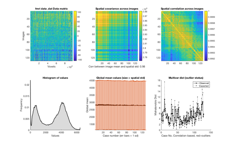
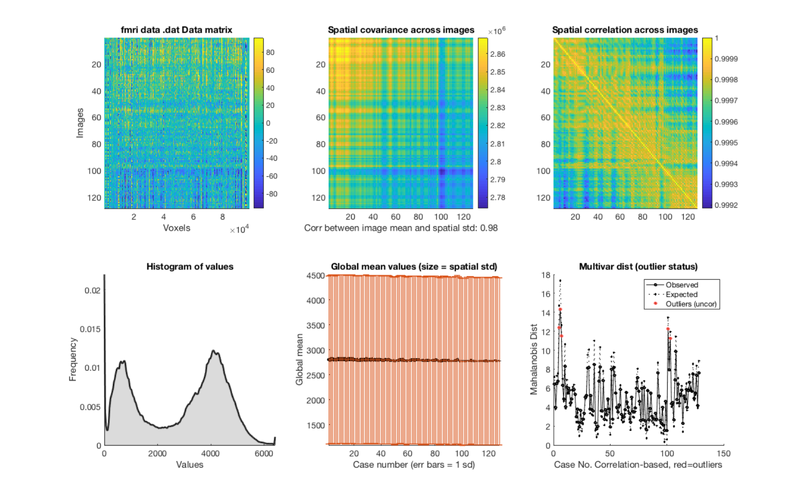
% Load one subject's data file into an object.
i = 1;
dat = fmri_data(imgs{i});

plot(dat)
drawnow, snapnow

% remove the task effects from each voxel in the dataset
% except the intercept (the last column)
% you wouldn't have to do this for resting-state data, but for this demo,
% we're using task data for convenience.
resid_data = dat.dat' - X.X(:, 1:end-1) * PX(1:end-1, :) * dat.dat';

% add the data back into the object
dat.dat = resid_data';

wh_outliers = plot(dat);
drawnow, snapnow
Using default mask: /Users/torwager/Dropbox (Dartmouth College)/Matlab_code_external/spm12/toolbox/FieldMap/brainmask.nii
loading mask. mapping volumes.
checking that dimensions and voxel sizes of volumes are the same.
Pre-allocating data array. Needed: 50137088 bytes
Loading image number:   128
Elapsed time is 0.858601 seconds.
Image names entered, but fullpath attribute is empty. Getting path info.
.fullpath should have image name for each image column in .dat
Attempting to expand image filenames in case image list is unexpanded 4-D images
Calculating mahalanobis distances to identify extreme-valued images
Retained 5 components for mahalanobis distance
Expected 50% of points within 50% normal ellipsoid, found 57.03%
Expected 6.40 outside 95% ellipsoid, found   0

Potential outliers based on mahalanobis distance:
Bonferroni corrected: 0 images		Cases
Uncorrected: 0 images		Cases

Outliers:
Outliers after p-value correction:
Image numbers:

Image numbers, uncorrected:
Warning: Ignoring extra legend entries.
Grouping contiguous voxels:   1 regions
Grouping contiguous voxels:   1 regions
Grouping contiguous voxels:   1 regions

ans =

  128×1 logical array

   0
   0
   0
   0
   0
   0
   0
   0
   0
   0
   0
   0
   0
   0
   0
   0
   0
   0
   0
   0
   0
   0
   0
   0
   0
   0
   0
   0
   0
   0
   0
   0
   0
   0
   0
   0
   0
   0
   0
   0
   0
   0
   0
   0
   0
   0
   0
   0
   0
   0
   0
   0
   0
   0
   0
   0
   0
   0
   0
   0
   0
   0
   0
   0
   0
   0
   0
   0
   0
   0
   0
   0
   0
   0
   0
   0
   0
   0
   0
   0
   0
   0
   0
   0
   0
   0
   0
   0
   0
   0
   0
   0
   0
   0
   0
   0
   0
   0
   0
   0
   0
   0
   0
   0
   0
   0
   0
   0
   0
   0
   0
   0
   0
   0
   0
   0
   0
   0
   0
   0
   0
   0
   0
   0
   0
   0
   0
   0

Calculating mahalanobis distances to identify extreme-valued images
Warning: Columns of X are linearly dependent to within machine precision.
Using only the first 118 components to compute TSQUARED.
Retained 5 components for mahalanobis distance
Expected 50% of points within 50% normal ellipsoid, found 53.91%
Expected 6.40 outside 95% ellipsoid, found   5

Potential outliers based on mahalanobis distance:
Bonferroni corrected: 0 images		Cases
Uncorrected: 5 images		Cases 5 6 7 101 103

Outliers:
Outliers after p-value correction:
Image numbers:

Image numbers, uncorrected: 5 6 7 101 103
Warning: Ignoring extra legend entries.
Grouping contiguous voxels:   1 regions
Grouping contiguous voxels:   1 regions
Grouping contiguous voxels:   1 regions
Preprocess the dataset
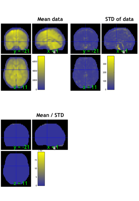
We notice some slow drift, and some potential outliers Run canlab_connectivity_preproc, which runs a series of preprocessing steps: Steps in order [with defaults]: 1. Remove nuisance covariates (and linear trend if requested) 2. Remove ventricle and white matter - default: uses canonical images with eroded MNI-space masks for these tissue compartments 3. High/low/bandpass filter on both data and covs before regression (plot) 4. Residualization using regression (plot) 5. (optional) Run additional GLM using the same additional preprocessing 6. Windsorize based on distribution of full data matrix (plot) 7. Extract region-by-region average ROI or pattern expression data
TR = 2.5;  % Repetition time between images
[preprocessed_dat] = canlab_connectivity_preproc(dat, 'vw', 'windsorize', 3, 'bpf', [.008 .25], TR);

drawnow, snapnow
===============================================================
Canlab_connectivity_preproc: starting preprocessing ...
::: removing ventricle & white matter signal ...
Extracting from gray_matter_mask.nii.
Extracting from canonical_white_matter_thrp5_ero1.nii.
Extracting from canonical_ventricles_thrp5_ero1.nii.
::: temporal filtering brain data...
::: temporal filtering covariates ...
Windsorized data matrix to 3 STD; adjusted 148713 values, 1.2% of values
Done: data preprocessing in 1.1e+01 sec.

---------------------------------------------------------------

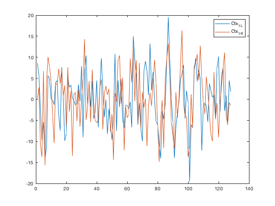
Extract and plot left vs. right M1 (motor) time series
This essentially reproduces the analysis in Biswal 1995
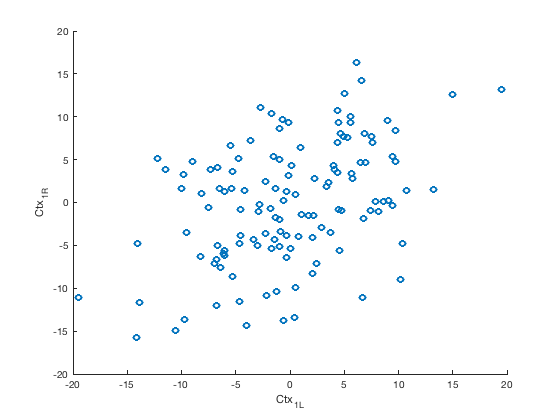
% Create a sub-atlas of regions whose labels match 'Ctx_1_'
m1_bilat = select_atlas_subset(atlas_obj, {'Ctx_1_'});

m1_bilat.labels

% Extract the timeseries in the 'seed' region for this dataset
m1_bilat_timeseries = extract_data(m1_bilat, preprocessed_dat);

% Plot the time series

figure; plot(m1_bilat_timeseries)
legend(m1_bilat.labels)

figure; scatter(m1_bilat_timeseries(:, 1), (m1_bilat_timeseries(:, 2)));
xlabel(m1_bilat.labels{1})
ylabel(m1_bilat.labels{2})
ans =

  1×2 cell array

    {'Ctx_1_L'}    {'Ctx_1_R'}

Resampling data object to space defined by atlas object.
Do a simple seed-based connectivity
% Load an atlas object to use to define the regions in the brainpathway object
atlas_obj = load_atlas('canlab2018_2mm');

m1 = select_atlas_subset(atlas_obj, {'Ctx_1_R'});

% Extract the timeseries in the 'seed' region for this dataset
m1_timeseries = extract_data(m1, preprocessed_dat);


% Assign seed region to .X field (design matrix) in data object, and run
% regression of this time series on all voxels
preprocessed_dat.X = m1_timeseries;

out = regress(preprocessed_dat);

% Regression method for fmri_data object
%
% Regress dat.X on dat.dat at each voxel, and return voxel-wise statistic
% images. Each column of dat.X is a predictor in a multiple regression,
% and the intercept is automatically added as the last column.

drawnow, snapnow

% The t-map for M1 connectivity is stored in the out.t, which has multiple
% images (one for the seed, and one for the intercept). We'll save the
% first one:

m1_t_map = get_wh_image(out.t, 1);

% now we can re-threshold it however we want:

m1_t_map = threshold(m1_t_map, .001, 'unc');

% display the map
create_figure('slices'); axis off
montage(m1_t_map)
drawnow, snapnow
Loading atlas: CANlab_combined_atlas_object_2018_2mm.mat
Resampling data object to space defined by atlas object.
Analysis:
----------------------------------
Design matrix warnings:
----------------------------------
No intercept detected, adding intercept to last column of design matrix
Warning:  Predictors are not centered -- intercept is not interpretable as stats for average subject

----------------------------------
Running regression: 97924 voxels. Design: 128 obs,   2 regressors, intercept is last

Predicting exogenous variable(s) in dat.X using brain data as predictors, mass univariate
Running in OLS Mode
Model run in 0 minutes and 0.23 seconds

Image   1
144 contig. clusters, sizes   1 to 17278
Positive effect: 17910 voxels, min p-value: 0.00000000
Negative effect: 239 voxels, min p-value: 0.00000012

Image   2
144 contig. clusters, sizes   1 to 17278
Positive effect:   0 voxels, min p-value: 0.16930103
Negative effect:   0 voxels, min p-value: 0.11178017
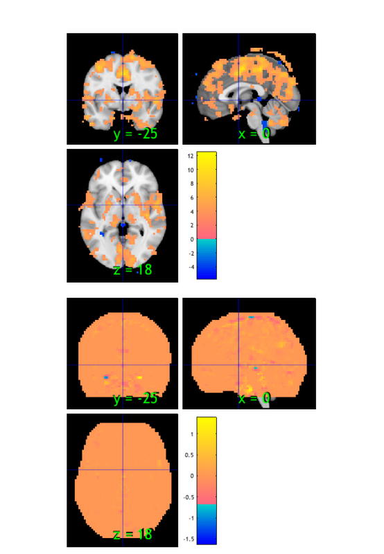
Image   1
144 contig. clusters, sizes   1 to 17278
Positive effect: 17910 voxels, min p-value: 0.00000000
Negative effect: 239 voxels, min p-value: 0.00000012
Setting up fmridisplay objects
Grouping contiguous voxels: 144 regions
sagittal montage: 572 voxels displayed, 17577 not displayed on these slices
sagittal montage: 641 voxels displayed, 17508 not displayed on these slices
sagittal montage: 744 voxels displayed, 17405 not displayed on these slices
axial montage: 3492 voxels displayed, 14657 not displayed on these slices
axial montage: 4069 voxels displayed, 14080 not displayed on these slices

ans =

  fmridisplay with properties:

            overlay: '/Users/torwager/Documents/GitHub/CanlabCore/CanlabCore/canlab_canonical_brains/Canonical_brains_surfaces/keuken_2014_enhanced_for_underlay.img'
              SPACE: [1×1 struct]
    activation_maps: {[1×1 struct]}
            montage: {1×5 cell}
            surface: {}
          orthviews: {}
            history: {}
    history_descrip: []
    additional_info: ''
Create a brainpathway object
Now we will use another object class, a "brainpathway" object This object class has specialized tools for handling connectivity and graphs.
% Show some of the methods (ignore 'static methods')
methods(brainpathway)

% This is a special type of object: When you operate on the object ("b" below),
% it changes the values everywhere, automatically. So you don't have to pass
% the object (b) in or out of functions. If you want to create a copy of
% the object, use the copy() method, e.g., b_copy = copy(b)

% Load an atlas object to use to define the regions in the brainpathway object
atlas_obj = load_atlas('canlab2018_2mm');

% Create the object using this atlas
 b = brainpathway(atlas_obj);      % Construct a brainpathway object from an atlas object, here "pain_pathways"

% b.region_atlas stores the atlas object within the brainpathways object
% you can assign a new atlas to change it.
% b.region_atlas.labels has all the labels for the regions.

b.region_atlas.labels(1:5)
Loading atlas: CANlab_combined_atlas_object_2018_2mm.mat
Initializing nodes to match regions.

Methods for class brainpathway:

attach_voxel_data                      find_node_indices
brainpathway                           plot_connectivity
brainpathway2fmri_data                 reorder_regions_by_node_cluster
cluster_region_subset_by_connectivity  seed_connectivity
cluster_regions                        select_atlas_subset
cluster_voxels                         threshold_connectivity
copy
degree_calc

Static methods:

intialize_nodes                        update_region_connectivity
update_node_connectivity               update_region_data
update_node_data

Call "methods('handle')" for methods of brainpathway inherited from handle.

Loading atlas: CANlab_combined_atlas_object_2018_2mm.mat
Initializing nodes to match regions.

ans =

  1×5 cell array

  Columns 1 through 4

    {'Ctx_V1_L'}    {'Ctx_V1_R'}    {'Ctx_MST_L'}    {'Ctx_MST_R'}

  Column 5

    {'Ctx_V6_L'}
Assign the subject's data to the object and calculate connectivity
When we do assign voxel-wise data to the object, it will automatically extract region averages for each parcel in the atlas and automatically calculate connectivity values
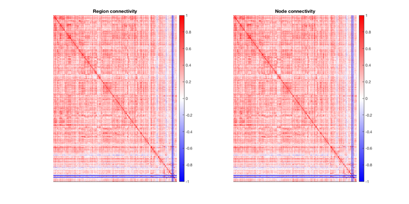
% First sample data to the space of the atlas
preprocessed_dat = resample_space(preprocessed_dat, atlas_obj);

% Now attach it to the brainpathway object (b) and calculate connectivity
b.voxel_dat = preprocessed_dat.dat;  % This calculates connectivity matrix and more when data are assigned

% Now we have:
% b.connectivity.regions.r  : Correlation matrices for all pairs of regions
% b.connectivity.regions.p  : P-values for correlations (assuming independent noise)

% And we can visualize this:
plot_connectivity(b)
drawnow, snapnow
Updating node response data.
Updating obj.connectivity.nodes.
Updating obj.connectivity.nodes.
Updating region averages.
Updating obj.connectivity.regions.
Warning: Error occurred while executing the listener callback for the
brainpathway class voxel_dat property PostSet event:
A dot name structure assignment is illegal when the structure is empty.  Use a
subscript on the structure.

Error in brainpathway.update_region_data (line 817)
            obj.data_quality.tSNR = mean(obj.region_dat) ./ std(obj.region_dat);
            % if data is mean-centered, will be meaningless

Error in brainpathway>@(src,evt)brainpathway.update_region_data(obj,src,evt)
(line 403)
            obj.listeners = addlistener(obj,'voxel_dat', 'PostSet',  @(src, evt)
            brainpathway.update_region_data(obj, src, evt));

Error in brainomics_connectivity_demo (line 188)
b.voxel_dat = preprocessed_dat.dat;  % This calculates connectivity matrix and
more when data are assigned

Error in evalmxdom>instrumentAndRun (line 115)
text = evalc(evalstr);

Error in evalmxdom (line 21)
[data,text,laste] =
instrumentAndRun(file,cellBoundaries,imageDir,imagePrefix,options);

Error in publish

Error in canlab_help_publish (line 26)
publish(pubfilename, p)

ans =

  struct with fields:

            r: [489×489 single]
            p: [489×489 double]
          sig: [489×489 logical]
    var_names: {}
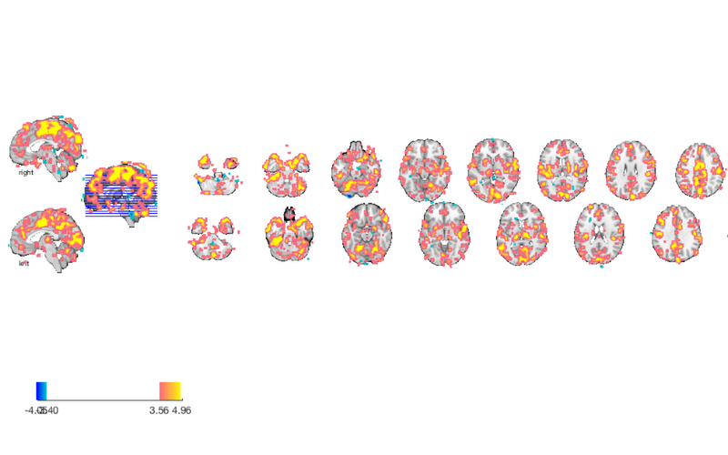
Do a seed connectivity analysis
...with one or more seeds, specified by the atlas labels
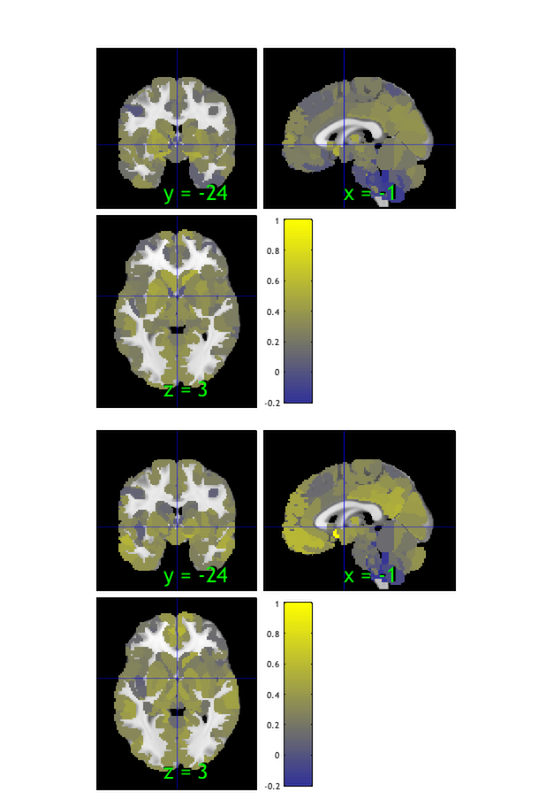
% Calculate correlation maps with all network averages in right M1 (primary
% motor cortex)
fmri_dat_connectivity_maps = seed_connectivity(b, {'Ctx_1_R'});

% Calculate correlation maps with all network averages containing 'NAC' in the label
fmri_dat_connectivity_maps = seed_connectivity(b, {'NAC'});

% Visualize the resulting maps, one per seed
orthviews(fmri_dat_connectivity_maps);
Calculating correlations between region averages and seed regions.
Calculating correlations between region averages and seed regions.
Grouping contiguous voxels:   1 regions
Grouping contiguous voxels:   1 regions