Contents
Basic Image Visualization
Using Basic Plot Methods (plot, orthviews, and montage) to Examine a Dataset
Objects can have methods with intuitive names, some of which overlap with names of functions in Matlab or other toolboxes. fmri_data.plot() is one of these. When you call plot() and pass in an fmri_data object, you invoke the fmri_data object method, and a special plot for fmri_data objects is produced.
You can list methods for an object class (e.g., fmri_data) by typing:
methods(fmri_data)
You can get help for a method by typing help class name.<method name> e.g., help fmri_data.plot
The plot() method takes an fMRI data object as a parameter and produces an SPM Orthview presentation along with 6 plots of the data.
The plot method expects an fMRI data object to be passed in. We can create an fMRI data object using the emotion regulation dataset via the following code:
[image_obj, networknames, imagenames] = load_image_set('emotionreg', 'noverbose');
Once created, we can pass this data object to the plot function to get the entire set of outputs, including Matlab console output regarding outliers and corresponding data visualizations, using the simple command:
plot(image_obj);
Calculating mahalanobis distances to identify extreme-valued images
Retained 8 components for mahalanobis distance
Expected 50% of points within 50% normal ellipsoid, found 46.67%
Expected 1.50 outside 95% ellipsoid, found   1

Potential outliers based on mahalanobis distance:
Bonferroni corrected: 0 images		Cases
Uncorrected: 1 images		Cases 27

Outliers:
Outliers after p-value correction:
Image numbers:

Image numbers, uncorrected: 27
Warning: Ignoring extra legend entries.
Grouping contiguous voxels:   1 regions
Grouping contiguous voxels:   1 regions
Grouping contiguous voxels:   1 regions
Explaining the output
The help file for fmri_data.plot did object has more information about the plots:
e.g., help fmri_data.plot
e.g., help image_obj.plot
help fmri_data.plot
Plot means by condition
plot(fmri_data_object, 'means_for_unique_Y')
:Inputs:
Plot methods:
- plot data matrix
- plot(fmri_data_object)
:Usage:
::
plot(fmridat, [plotmethod])
:Outputs:
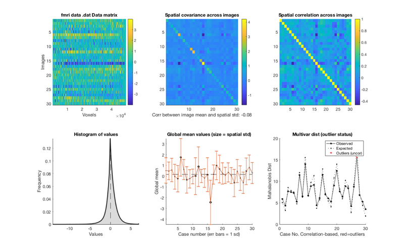
6 plots and an SPM orthviews presentation of the data. In the below
and elsewhere, "image" connotes a 3D brain volume captured every TR.
**subplot 1:**
Data matrix (top left). Also called a "carpet plot" in neuroimaging.
The color reflects the intensity of signal in each voxel (column)
for each image (row).
Here you can look for images that are bright or dark across
the image, which would indicate a global shift in values or difference
in scale across the images (rows).
These can be produced by artifacts that are broadly spatially distributed,
or by scanner drift. Most datasets have some of these.
This plot can also show that the pattern across voxels in one row (image)
may be different than another, highlighting a difference in the spatial pattern.
If you are plotting a time series dataset from one participant, unusual images
could result from physiological noise, head movement, or other
scanner artifacts. They could reflect after-effects of non-linear
interactions across these, or a change in the images after a
participant has moved their head to a new position.
If you are plotting a group dataset with one contrast image per
participant (i.e., what you would subject to a group analysis),
standard statistical assumptions include that observations
(participants) are all on the same scale, with the same variance.
It is common for these assumptions to be violated, and you can
sometimes see these violations here.
Lastly, the range shown in the color bar on the right side of this plot
will be quite large if there are large outliers in the data.
The units are in contrast unit values, but it is important to check if a
few extreme values are forcing all other values to be in the middle of the scale.
In this case, there will be very little color variation in the plot, which is a
"red flag" indicating outliers or extreme values.
Other plots show you different representations of this dataset,
in ways that make it easier to see some of its properties.
**subplots 2 and 3:**
Covariance and Correlation Matrices (Top Middle/Top Left):
These plots both show similarity across images. Both should show bright main
diagonals and off-diagonals that are non zero or generally positive, depending
on the dataset.
Covariance Matrix: $\frac{{X}'X}{n-1}$, X is mean-centered, n is number of rows in X
The diagonal reflects the image variance, shows whether the variances
of each image are equal. If the variances are all of approximately the same scale,
the diagonal will be a single color.
Correlation Matrix $\frac{{X}'X}{n-1}$, colums of X are Z-scored, n is number of rows in X
This plot shows the correlation between each image and the others.
Now, the main diagonal will always be one because each image is
perfectly correlated with itself. The off-diagonals should be positive
if the images are similar to one another.
**subplot 4:**
Histogram (Bottom Left): A histogram of values across all images and voxels.
Depending on your input images, low values could reflect out-of-brain voxels,
as there is no signal there. Values of exactly 0 are excluded as missing data
in all image operations.
For a group dataset (e.g., contrast images), it is expected that
the distribution of contrast values will have roughly mean 0.
There are other tools for looking at this distribution for each individual
image in the dataset, and each image x tissue type (assuming
MNI-space images). See help fmri_data.histogram.
**subplot 5:**
The Global Mean Values (Bottom Middle) for each image.
The means ought to be similar to one another. Ideally, these means
will all be in a similar range. The error bars show one standard deviation.
each point is an image. The point's X value is the mean
intensity of every voxel in that image, and the Y value is the
stdev of intensities for all voxels in that image.
**subplot 6:**
Mahalanobis Distance (Bottom Right) is a measure of how far away each
image is from the rest in the sample. This a standard measure of multivariate
distance for each of a set of multivariate observations (here, images).
The larger the distance, the more dissimilar it is from other images.
High values generally indicate extreme values/potential outliers, but
in any normally distributed dataset, there are going to be some values
that lie farther out. Also note that what to do about extreme values
can be complex, and there is much discussion about how to handle
them.
Potential outliers are identified using fmri_data.mahal.
To identify outliers, we assume that the points are distributed according
to a chi-square distribution. The expected distance is based on multivariate
normally distributed data for the percentile of the dataset that corresponds
to each image. even the most extreme values may not be greater than what
one expects by chance. The analysis produces p-values at uncorrected and
Bonferroni-corrected levels, and any image that is marked as an outlier
is one that exceeds the expected value with a p-value of less than 0.05.
Those will be marked in darker red. Anything considered to be an outlier with
p < 0.05 Bonferroni corrected will be marked with an even darker red.
The outliers from this plot are returned to the workspace as output.
Note: Outlier identification here does not use global values, only Mahalanobis distance.
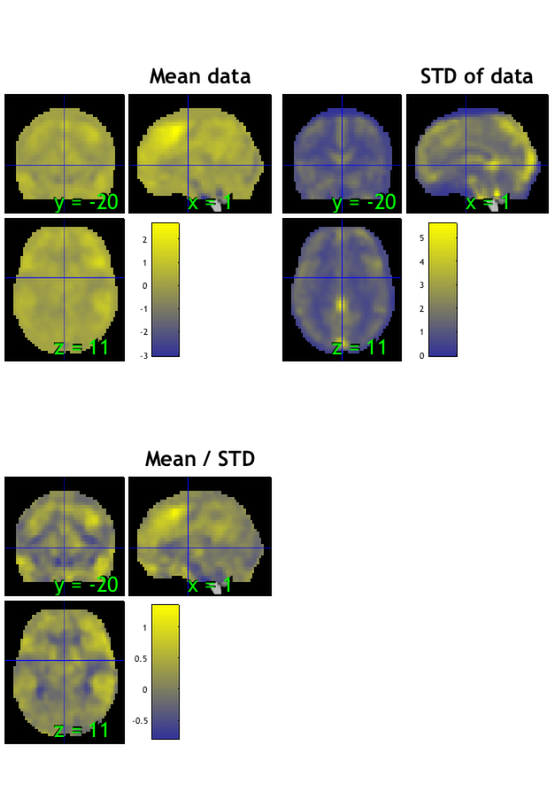
**Orthviews:**
SPM Orthviews: These use the spm_orthviews function from SPM software.
The X,Y, and Z coordinates correspond to the distance in millimeters
from the set origin. Three images are shown:
- The mean image is the voxel-wise average across images in the dataset
- The STD image is the voxel-wise standard deviation across images in the dataset
- The mean/STD image is a simple estimate of effect size (Cohen's D) for every voxel.
If a contrast with one image per person is passed to plot(), this plot gives you
the effect size in a simple group analysis (e.g., one-sample t-test) across
the brain. It is reasonable to use this plot to look for distortions such as high values for means and mean/STDs in the ventricles.
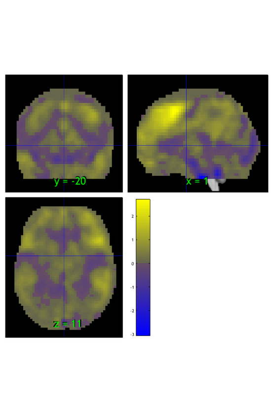
Use Orthviews to visualize the mean image
Some other commonly used methods to display images are the orthviews() and montage() methods. fmri_data objects have these methods, and other object classes do to, like the statistic_image, atlas, and region classes.
First, let's create a mean image for the dataset:
m = mean(image_obj);
orthviews(m);
drawnow, snapnow
Grouping contiguous voxels: 1 regions
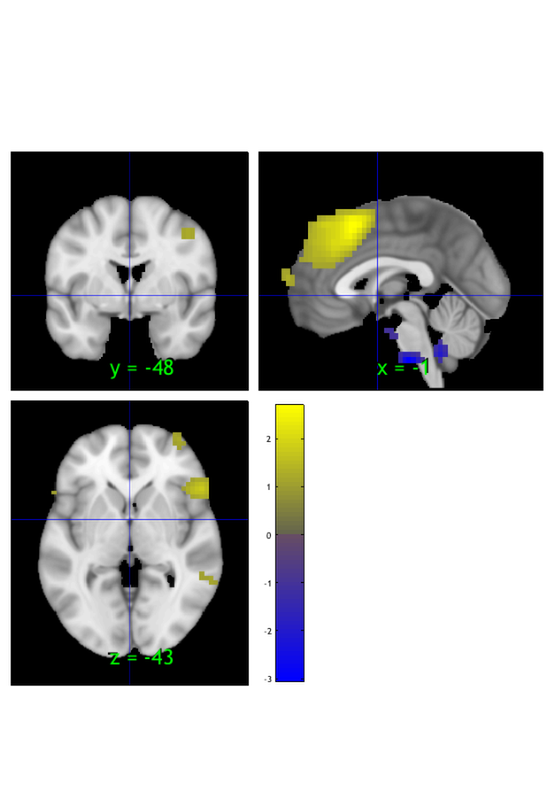
Threshold and display
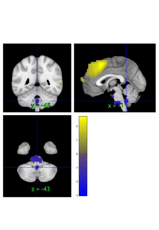
let's threshold it using the threshold() method. Here we'll exclude values between -1 and 1 and view the extreme values:
m = threshold(m, [-1 1], 'raw-outside');
orthviews(m);
drawnow, snapnow
Keeping vals outside of -1.000 to 1.000: 1428 elements remain
Grouping contiguous voxels:  22 regions
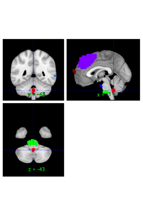
Create and display a region object
We can create a region class object, another type of object, from the thresholded image. This has additional info and options about each contiguous 'blob' in the suprathreshold map:
r = region(m);
orthviews(r);
drawnow, snapnow
Grouping contiguous voxels: 22 regions
Orthviews options
Orthviews methods have a range of options. They use the cluster_orthviews function, which uses spm_orthviews See help cluster_orthviews for options.
Let's try one that visualizes each contiguous blob in a different, solid color:
orthviews(r, 'unique', 'solid');
drawnow, snapnow
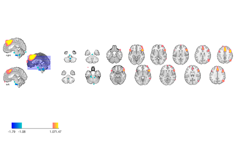
Use montage to visualize the thresholded mean image
Sometimes, we want to view map that shows a canonical range of slices. This is really useful for producing standard output for papers Arguably, one should always view and publish montage maps showing all slices, so as to show the "whole picture" and not omit any results.
You can customize this a lot, as it uses the fmridisplay() object class, which allows you to add custom montages (in axial, saggital, and coronal orientations, add blobs of various types, and remove them and re-plot. See help fmridisplay and help fmridisplay.addblobs for more details.
For now, we'll just stick to a basic plot. We'll first create an empty figure,then plot the montage on it.
create_figure('montage'); axis off;
montage(m);
drawnow, snapnow

% We've already thresholded it, so it'll use the previous threshold.
% however, we can re-threshold the image and redisplay it as well.
Setting up fmridisplay objects
This takes a lot of memory, and can hang if you have too little.
Grouping contiguous voxels:  22 regions
sagittal montage:  64 voxels displayed, 1364 not displayed on these slices
sagittal montage: 120 voxels displayed, 1308 not displayed on these slices
sagittal montage: 145 voxels displayed, 1283 not displayed on these slices
axial montage: 346 voxels displayed, 1082 not displayed on these slices
axial montage: 470 voxels displayed, 958 not displayed on these slices
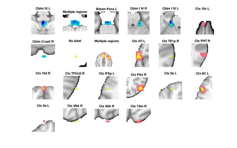
Use montage to visualize each blob in a thresholded map
A really useful thing to do is to take a region object, often from a thresholded map, and visualize each region. the montage() methods also have a number of options. Let's try one, 'regioncenters', that plots each blob (region) on a separate slice.
Furthermore, we can use the 'colormap' option to view the regions with colors mapped to their associated values, e.g., hot colors for positive values and cool colors for negative values.
Finally, we might want to assign names to each region based on an atlas. We'll do that before plotting, so that the names appear on the plots. These names are saved in the r(i).shorttitle field, for each region i. The region.table() method automatically labels them as well. You can customize the atlas used; the default is the 'canlab2018_2mm' atlas (see help load_atlas for more info.)
r = autolabel_regions_using_atlas(r);

montage(r, 'regioncenters', 'colormap');
drawnow, snapnow

% Note that some large regions may span multiple areas.
% This can happen if the various regions are connected by contiguous
% suprathreshold voxels.

Explore on your own
1. Try to re-threshold the image using some values you choose and re-plot. Look at the help for more options on thresholding. and pick one. What do you see? Try to plot only voxels with positive values in the mean image.
2. Try to bring up only one region from the region object (r) in orthviews. Can you visualize it in all three views?
3. Try using a couple of other display options in the montage() and orthviews() methods. What do you see?
% That's it for this section!!