Perform a voxel-wise t-test
In this example we perform a second level analysis on first level statistical parametric maps. Specifically we use a t-test to obtain an ordinary least squares estimate for the group level parameter.
The example uses the emotion regulation data provided with CANlab_Core_Tools. This dataset consists of a set of contrast images for 30 subjects from a first level analysis. The contrast is [reappraise neg vs. look neg], reappraisal of negative images vs. looking at matched negative images.
These data were published in: Wager, T. D., Davidson, M. L., Hughes, B. L., Lindquist, M. A., Ochsner, K. N.. (2008). Prefrontal-subcortical pathways mediating successful emotion regulation. Neuron, 59, 1037-50.
By the end of this example we will have regenerated the results of figure 2A of this paper.
Contents
Executive summary of the whole analysis
As a summary, here is a complete set of commands to load the data and run the entire analysis:
   img_obj = load_image_set('emotionreg');         % Load a dataset
   t = ttest(img_obj);                             % Do a group t-test
   t = threshold(t, .05, 'fdr', 'k', 10);          % Threshold with FDR q < .05 and extent threshold of 10 contiguous voxels
% Show regions and print a table with labeled regions: montage(t); drawnow, snapnow; % Show results on a slice display r = region(t); % Turn t-map into a region object with one element per contig region table(r); % Print a table of results using new region names
Here a graphical description of what it does:
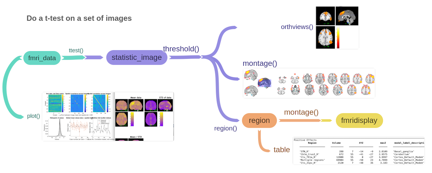
Now, let's walk through it step by step, with a few minor additions.
Load sample data
% We can load this data using load_image_set(), which produces an fmri_data
% object. Data loading exceeds the scope of this tutorial, but a more
% indepth demosntration may be provided by load_a_sample_dataset.m

[image_obj, networknames, imagenames] = load_image_set('emotionreg');
Loaded images:
/Users/torwager/Documents/GitHub/CanlabCore/CanlabCore/Sample_datasets/Wager_et_al_2008_Neuron_EmotionReg/Wager_2008_emo_reg_vs_look_neg_contrast_images.nii
/Users/torwager/Documents/GitHub/CanlabCore/CanlabCore/Sample_datasets/Wager_et_al_2008_Neuron_EmotionReg/Wager_2008_emo_reg_vs_look_neg_contrast_images.nii
/Users/torwager/Documents/GitHub/CanlabCore/CanlabCore/Sample_datasets/Wager_et_al_2008_Neuron_EmotionReg/Wager_2008_emo_reg_vs_look_neg_contrast_images.nii
/Users/torwager/Documents/GitHub/CanlabCore/CanlabCore/Sample_datasets/Wager_et_al_2008_Neuron_EmotionReg/Wager_2008_emo_reg_vs_look_neg_contrast_images.nii
/Users/torwager/Documents/GitHub/CanlabCore/CanlabCore/Sample_datasets/Wager_et_al_2008_Neuron_EmotionReg/Wager_2008_emo_reg_vs_look_neg_contrast_images.nii
/Users/torwager/Documents/GitHub/CanlabCore/CanlabCore/Sample_datasets/Wager_et_al_2008_Neuron_EmotionReg/Wager_2008_emo_reg_vs_look_neg_contrast_images.nii
/Users/torwager/Documents/GitHub/CanlabCore/CanlabCore/Sample_datasets/Wager_et_al_2008_Neuron_EmotionReg/Wager_2008_emo_reg_vs_look_neg_contrast_images.nii
/Users/torwager/Documents/GitHub/CanlabCore/CanlabCore/Sample_datasets/Wager_et_al_2008_Neuron_EmotionReg/Wager_2008_emo_reg_vs_look_neg_contrast_images.nii
/Users/torwager/Documents/GitHub/CanlabCore/CanlabCore/Sample_datasets/Wager_et_al_2008_Neuron_EmotionReg/Wager_2008_emo_reg_vs_look_neg_contrast_images.nii
/Users/torwager/Documents/GitHub/CanlabCore/CanlabCore/Sample_datasets/Wager_et_al_2008_Neuron_EmotionReg/Wager_2008_emo_reg_vs_look_neg_contrast_images.nii
/Users/torwager/Documents/GitHub/CanlabCore/CanlabCore/Sample_datasets/Wager_et_al_2008_Neuron_EmotionReg/Wager_2008_emo_reg_vs_look_neg_contrast_images.nii
/Users/torwager/Documents/GitHub/CanlabCore/CanlabCore/Sample_datasets/Wager_et_al_2008_Neuron_EmotionReg/Wager_2008_emo_reg_vs_look_neg_contrast_images.nii
/Users/torwager/Documents/GitHub/CanlabCore/CanlabCore/Sample_datasets/Wager_et_al_2008_Neuron_EmotionReg/Wager_2008_emo_reg_vs_look_neg_contrast_images.nii
/Users/torwager/Documents/GitHub/CanlabCore/CanlabCore/Sample_datasets/Wager_et_al_2008_Neuron_EmotionReg/Wager_2008_emo_reg_vs_look_neg_contrast_images.nii
/Users/torwager/Documents/GitHub/CanlabCore/CanlabCore/Sample_datasets/Wager_et_al_2008_Neuron_EmotionReg/Wager_2008_emo_reg_vs_look_neg_contrast_images.nii
/Users/torwager/Documents/GitHub/CanlabCore/CanlabCore/Sample_datasets/Wager_et_al_2008_Neuron_EmotionReg/Wager_2008_emo_reg_vs_look_neg_contrast_images.nii
/Users/torwager/Documents/GitHub/CanlabCore/CanlabCore/Sample_datasets/Wager_et_al_2008_Neuron_EmotionReg/Wager_2008_emo_reg_vs_look_neg_contrast_images.nii
/Users/torwager/Documents/GitHub/CanlabCore/CanlabCore/Sample_datasets/Wager_et_al_2008_Neuron_EmotionReg/Wager_2008_emo_reg_vs_look_neg_contrast_images.nii
/Users/torwager/Documents/GitHub/CanlabCore/CanlabCore/Sample_datasets/Wager_et_al_2008_Neuron_EmotionReg/Wager_2008_emo_reg_vs_look_neg_contrast_images.nii
/Users/torwager/Documents/GitHub/CanlabCore/CanlabCore/Sample_datasets/Wager_et_al_2008_Neuron_EmotionReg/Wager_2008_emo_reg_vs_look_neg_contrast_images.nii
/Users/torwager/Documents/GitHub/CanlabCore/CanlabCore/Sample_datasets/Wager_et_al_2008_Neuron_EmotionReg/Wager_2008_emo_reg_vs_look_neg_contrast_images.nii
/Users/torwager/Documents/GitHub/CanlabCore/CanlabCore/Sample_datasets/Wager_et_al_2008_Neuron_EmotionReg/Wager_2008_emo_reg_vs_look_neg_contrast_images.nii
/Users/torwager/Documents/GitHub/CanlabCore/CanlabCore/Sample_datasets/Wager_et_al_2008_Neuron_EmotionReg/Wager_2008_emo_reg_vs_look_neg_contrast_images.nii
/Users/torwager/Documents/GitHub/CanlabCore/CanlabCore/Sample_datasets/Wager_et_al_2008_Neuron_EmotionReg/Wager_2008_emo_reg_vs_look_neg_contrast_images.nii
/Users/torwager/Documents/GitHub/CanlabCore/CanlabCore/Sample_datasets/Wager_et_al_2008_Neuron_EmotionReg/Wager_2008_emo_reg_vs_look_neg_contrast_images.nii
/Users/torwager/Documents/GitHub/CanlabCore/CanlabCore/Sample_datasets/Wager_et_al_2008_Neuron_EmotionReg/Wager_2008_emo_reg_vs_look_neg_contrast_images.nii
/Users/torwager/Documents/GitHub/CanlabCore/CanlabCore/Sample_datasets/Wager_et_al_2008_Neuron_EmotionReg/Wager_2008_emo_reg_vs_look_neg_contrast_images.nii
/Users/torwager/Documents/GitHub/CanlabCore/CanlabCore/Sample_datasets/Wager_et_al_2008_Neuron_EmotionReg/Wager_2008_emo_reg_vs_look_neg_contrast_images.nii
/Users/torwager/Documents/GitHub/CanlabCore/CanlabCore/Sample_datasets/Wager_et_al_2008_Neuron_EmotionReg/Wager_2008_emo_reg_vs_look_neg_contrast_images.nii
/Users/torwager/Documents/GitHub/CanlabCore/CanlabCore/Sample_datasets/Wager_et_al_2008_Neuron_EmotionReg/Wager_2008_emo_reg_vs_look_neg_contrast_images.nii
Do a t-test
% Voxel-wise tests estimate parameters for each voxel independently. The
% fmri_data/ttest function performs this just like the native matlab
% ttest() function, and similarly returns a p-value and t-stat. Unlike the
% matlab ttest() function, fmri_data/ttest performs this for every voxel in
% the fmri_data object. All voxels are evaluated independently, but all are
% evaluated nonetheless. A statistic_image is returned.

t = ttest(image_obj);
One-sample t-test
Calculating t-statistics and p-values
Visualize the results
There are many options. See methods(statistic_image) and methods(region)
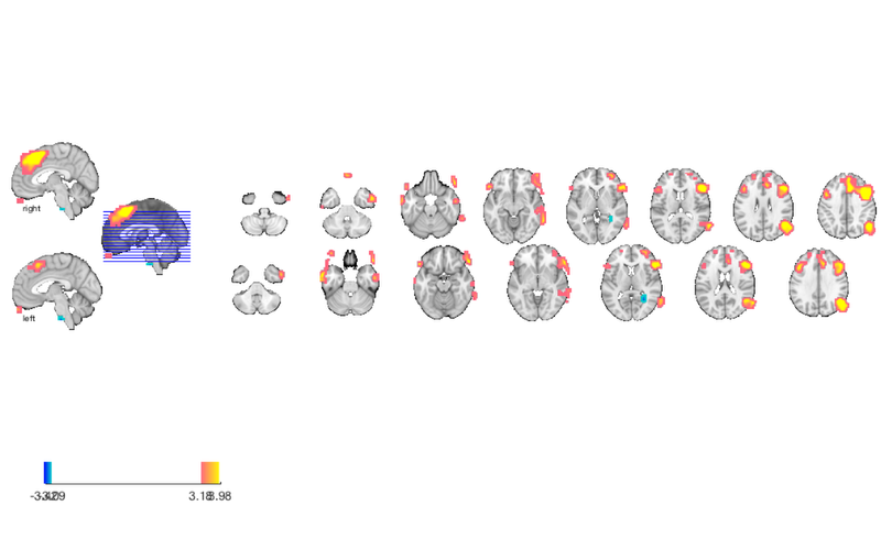
orthviews(t)
drawnow, snapnow;

% As can be seen, the ttest() result is unthresholded. The threshold
% function can be used to apply a desired alpha level using any of a number
% of methods. Here FDR is used to control for alpha=0.05. Note that no
% information is erased when performing thresholding on a statistic_image.

t = threshold(t, .05, 'fdr');
orthviews(t)
drawnow, snapnow;

% Many neuroimaging packages (e.g., SPM and FSL) do one-tailed tests
% (with one-tailed p-values) and only show you positive effects
% (i.e., relative activations, not relative deactivations).
% All the CANlab tools do two-sided tests, report two-tailed p-values.
% By default, hot colors (orange/yellow) will show activations, and cool
% colors (blues) show deactivations.

% We can also apply an "extent threshold" of > 10 contiguous voxels:

t = threshold(t, .05, 'fdr', 'k', 10);
orthviews(t)
drawnow, snapnow;

% montage is another visualization method. This function may require a
% relatively large amount of memory, depending on the resolution of the
% anatomical underlay image you use. We recommend around 8GB of free memory.
%
create_figure('montage'); axis off
montage(t)
drawnow, snapnow;
SPM12: spm_check_registration (v6245)              18:17:57 - 09/01/2020
========================================================================
Display <a href="matlab:spm_image('display','/Users/torwager/Documents/GitHub/CanlabCore/CanlabCore/canlab_canonical_brains/Canonical_brains_surfaces/keuken_2014_enhanced_for_underlay.img,1');">/Users/torwager/Documents/GitHub/CanlabCore/CanlabCore/canlab_canonical_brains/Canonical_brains_surfaces/keuken_2014_enhanced_for_underlay.img,1</a>

ans =

  1×1 cell array

    {1×1 struct}
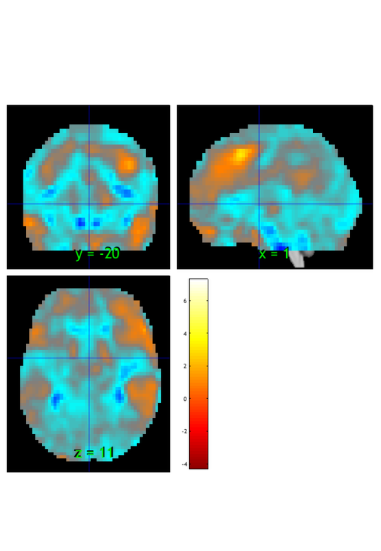
Image   1 FDR q < 0.050 threshold is 0.002549

Image   1
 27 contig. clusters, sizes   1 to 1472
Positive effect: 2502 voxels, min p-value: 0.00000000
Negative effect:  37 voxels, min p-value: 0.00022793

SPM12: spm_check_registration (v6245)              18:18:00 - 09/01/2020
========================================================================
Display <a href="matlab:spm_image('display','/Users/torwager/Documents/GitHub/CanlabCore/CanlabCore/canlab_canonical_brains/Canonical_brains_surfaces/keuken_2014_enhanced_for_underlay.img,1');">/Users/torwager/Documents/GitHub/CanlabCore/CanlabCore/canlab_canonical_brains/Canonical_brains_surfaces/keuken_2014_enhanced_for_underlay.img,1</a>

ans =

  1×1 cell array

    {1×27 struct}

Image   1 FDR q < 0.050 threshold is 0.002549

Image   1
  9 contig. clusters, sizes  10 to 1472
Positive effect: 2460 voxels, min p-value: 0.00000000
Negative effect:  32 voxels, min p-value: 0.00022793

SPM12: spm_check_registration (v6245)              18:18:01 - 09/01/2020
========================================================================
Display <a href="matlab:spm_image('display','/Users/torwager/Documents/GitHub/CanlabCore/CanlabCore/canlab_canonical_brains/Canonical_brains_surfaces/keuken_2014_enhanced_for_underlay.img,1');">/Users/torwager/Documents/GitHub/CanlabCore/CanlabCore/canlab_canonical_brains/Canonical_brains_surfaces/keuken_2014_enhanced_for_underlay.img,1</a>

ans =

  1×1 cell array

    {1×9 struct}

Setting up fmridisplay objects
This takes a lot of memory, and can hang if you have too little.
Grouping contiguous voxels:   9 regions
sagittal montage:  31 voxels displayed, 2461 not displayed on these slices
sagittal montage:  97 voxels displayed, 2395 not displayed on these slices
sagittal montage:  76 voxels displayed, 2416 not displayed on these slices
axial montage: 808 voxels displayed, 1684 not displayed on these slices
axial montage: 904 voxels displayed, 1588 not displayed on these slices

ans =

  fmridisplay with properties:

            overlay: '/Users/torwager/Documents/GitHub/CanlabCore/CanlabCore/canlab_canonical_brains/Canonical_brains_surfaces/keuken_2014_enhanced_for_underlay.img'
              SPACE: [1×1 struct]
    activation_maps: {[1×1 struct]}
            montage: {1×5 cell}
            surface: {}
          orthviews: {}
            history: {}
    history_descrip: []
    additional_info: ''
Print a table of results
% First, we'll have to convert to another object type, a "region object".
% This object groups voxels together into "blobs" (often of contiguous
% voxels). It does many things that other object types do, and inter-operates
% with them closely.  See methods(region) for more info.

% Create a region object called "r", with contiguous blobs from the
% thresholded t-map:

r = region(t);

% Print the table:

table(r);
Grouping contiguous voxels:   9 regions

____________________________________________________________________________________________________________________________________________
Positive Effects
          Region            Volume             XYZ            maxZ     modal_label_descriptions    Perc_covered_by_label    Atlas_regions_covered    region_index
    __________________    __________    _________________    ______    ________________________    _____________________    _____________________    ____________

    'Ctx_TE1a_R'                9864     55      0    -27    3.9997     'Cortex_Default_ModeA'              30                        2                   1
    'Multiple regions'         57152     55    -58     23    4.7899     'Cortex_Default_ModeA'               7                       10                   6
    'Multiple regions'         31664    -55     21      9    4.1824     'Cortex_Default_ModeB'               9                       10                   2
    'Multiple regions'    1.4038e+05     31     28     36    7.0345     'Cortex_Default_ModeB'               4                       38                   4
    'Ctx_9a_L'                  4336    -24     52     27     3.443     'Cortex_Default_ModeB'              35                        1                   7
    'Ctx_10v_L'                 3752     -3     58    -32     3.943     'Cortex_Limbic'                      7                        0                   3
    'No label'                   912    -45     52    -23    3.8446     'No description'                     0                        0                   5


Negative Effects
        Region        Volume          XYZ            maxZ       modal_label_descriptions     Perc_covered_by_label    Atlas_regions_covered    region_index
    ______________    ______    ________________    _______    __________________________    _____________________    _____________________    ____________

    'Bstem_Pons_L'     2016     -3    -24    -50    -3.6859    'Brainstem'                            22                        0                   8
    'Ctx_ProS_R'       2832     28    -48      9    -3.3405    'Cortex_Visual_Peripheral'             12                        0                   9


____________________________________________________________________________________________________________________________________________
Regions labeled by reference atlas CANlab_2018_combined

Volume: Volume of contiguous region in cubic mm.
MaxZ: Signed max over Z-score for each voxel.
Atlas_regions_covered: Number of reference atlas regions covered at least 25% by the region. This relates to whether the region covers
multiple reference atlas regions
Region: Best reference atlas label, defined as reference region with highest number of in-region voxels. Regions covering >25% of >5
regions labeled as "Multiple regions"
Perc_covered_by_label: Percentage of the region covered by the label.
Ref_region_perc: Percentage of the label region within the target region.
modal_atlas_index: Index number of label region in reference atlas
all_regions_covered: All regions covered >5% in descending order of importance

For example, if a region is labeled 'TE1a' and Perc_covered_by_label = 8, Ref_region_perc = 38, and Atlas_regions_covered = 17, this means
that 8% of the region's voxels are labeled TE1a, which is the highest percentage among reference label regions. 38% of the region TE1a is
covered by the region. However, the region covers at least 25% of 17 distinct labeled reference regions.

References for atlases:

Beliveau, Vincent, Claus Svarer, Vibe G. Frokjaer, Gitte M. Knudsen, Douglas N. Greve, and Patrick M. Fisher. 2015. “Functional
Connectivity of the Dorsal and Median Raphe Nuclei at Rest.” NeuroImage 116 (August): 187–95.
Bär, Karl-Jürgen, Feliberto de la Cruz, Andy Schumann, Stefanie Koehler, Heinrich Sauer, Hugo Critchley, and Gerd Wagner. 2016. ?Functional
Connectivity and Network Analysis of Midbrain and Brainstem Nuclei.? NeuroImage 134 (July):53?63.
Diedrichsen, Jörn, Joshua H. Balsters, Jonathan Flavell, Emma Cussans, and Narender Ramnani. 2009. A Probabilistic MR Atlas of the Human
Cerebellum. NeuroImage 46 (1): 39?46.
Fairhurst, Merle, Katja Wiech, Paul Dunckley, and Irene Tracey. 2007. ?Anticipatory Brainstem Activity Predicts Neural Processing of Pain
in Humans.? Pain 128 (1-2):101?10.
Fan 2016 Cerebral Cortex; doi:10.1093/cercor/bhw157
Glasser, Matthew F., Timothy S. Coalson, Emma C. Robinson, Carl D. Hacker, John Harwell, Essa Yacoub, Kamil Ugurbil, et al. 2016. A
Multi-Modal Parcellation of Human Cerebral Cortex. Nature 536 (7615): 171?78.
Keren, Noam I., Carl T. Lozar, Kelly C. Harris, Paul S. Morgan, and Mark A. Eckert. 2009. “In Vivo Mapping of the Human Locus Coeruleus.”
NeuroImage 47 (4): 1261–67.
Keuken, M. C., P-L Bazin, L. Crown, J. Hootsmans, A. Laufer, C. Müller-Axt, R. Sier, et al. 2014. “Quantifying Inter-Individual Anatomical
Variability in the Subcortex Using 7 T Structural MRI.” NeuroImage 94 (July): 40–46.
Krauth A, Blanc R, Poveda A, Jeanmonod D, Morel A, Székely G. (2010) A mean three-dimensional atlas of the human thalamus: generation from
multiple histological data. Neuroimage. 2010 Feb 1;49(3):2053-62. Jakab A, Blanc R, Berényi EL, Székely G. (2012) Generation of
Individualized Thalamus Target Maps by Using Statistical Shape Models and Thalamocortical Tractography. AJNR Am J Neuroradiol. 33:
2110-2116, doi: 10.3174/ajnr.A3140
Nash, Paul G., Vaughan G. Macefield, Iven J. Klineberg, Greg M. Murray, and Luke A. Henderson. 2009. ?Differential Activation of the Human
Trigeminal Nuclear Complex by Noxious and Non-Noxious Orofacial Stimulation.? Human Brain Mapping 30 (11):3772?82.
Pauli 2018 Bioarxiv: CIT168 from Human Connectome Project data
Pauli, Wolfgang M., Amanda N. Nili, and J. Michael Tyszka. 2018. ?A High-Resolution Probabilistic in Vivo Atlas of Human Subcortical Brain
Nuclei.? Scientific Data 5 (April): 180063.
Pauli, Wolfgang M., Randall C. O?Reilly, Tal Yarkoni, and Tor D. Wager. 2016. ?Regional Specialization within the Human Striatum for
Diverse Psychological Functions.? Proceedings of the National Academy of Sciences of the United States of America 113 (7): 1907?12.
Sclocco, Roberta, Florian Beissner, Gaelle Desbordes, Jonathan R. Polimeni, Lawrence L. Wald, Norman W. Kettner, Jieun Kim, et al. 2016.
?Neuroimaging Brainstem Circuitry Supporting Cardiovagal Response to Pain: A Combined Heart Rate Variability/ultrahigh-Field (7 T)
Functional Magnetic Resonance Imaging Study.? Philosophical Transactions. Series A, Mathematical, Physical, and Engineering Sciences 374
(2067). rsta.royalsocietypublishing.org. https://doi.org/10.1098/rsta.2015.0189.
Shen, X., F. Tokoglu, X. Papademetris, and R. T. Constable. 2013. “Groupwise Whole-Brain Parcellation from Resting-State fMRI Data for
Network Node Identification.” NeuroImage 82 (November): 403–15.
Zambreanu, L., R. G. Wise, J. C. W. Brooks, G. D. Iannetti, and I. Tracey. 2005. ?A Role for the Brainstem in Central Sensitisation in
Humans. Evidence from Functional Magnetic Resonance Imaging.? Pain 114 (3):397?407.

Note: Region object r(i).title contains full list of reference atlas regions covered by each cluster.
____________________________________________________________________________________________________________________________________________
More on getting help
% Help info is available on https://canlab.github.io/
% and in the CANlab help examples repository: https://github.com/canlab/CANlab_help_examples
% This contains a series of walkthroughs, including this one.

% You can get help for the main object types by typing this in Matlab:
% doc fmri_data (or doc any other object types)

% Also, more detailed help is available for each function using the "help" command.
% You can get help and options for any object method, like "table". But
% because the method names are simple and often overlap with other Matlab functions
% and toolboxes (this is OK for objects!), you will often want to specify
% the object type as well, as follows:

% help region.table
Write the t-map to disk
% Now we need to save our results. You can save the objects in your
% workspace or you can write your resulting thresholded map to an analyze
% file. The latter may be useful for generating surface projections using
% Caret or FreeSurfer for instance.
%
% Thresholding did not actually eliminate nonsignificant voxels from our
% statistic_image object (t). If we  simply write out that object, we will
% get t-statistics for all voxels.

t.fullpath = fullfile(pwd, 'example_t_image.nii');
write(t)

% If we use the 'thresh' option, we'll write thresholded values:
write(t, 'thresh')

t_reloaded = statistic_image(t.fullpath, 'type', 'generic');
orthviews(t_reloaded)
Writing:
/Users/torwager/Documents/GitHub/example_t_image.nii
Writing thresholded statistic image.
Writing:
/Users/torwager/Documents/GitHub/example_t_image.nii

SPM12: spm_check_registration (v6245)              18:18:12 - 09/01/2020
========================================================================
Display <a href="matlab:spm_image('display','/Users/torwager/Documents/GitHub/CanlabCore/CanlabCore/canlab_canonical_brains/Canonical_brains_surfaces/keuken_2014_enhanced_for_underlay.img,1');">/Users/torwager/Documents/GitHub/CanlabCore/CanlabCore/canlab_canonical_brains/Canonical_brains_surfaces/keuken_2014_enhanced_for_underlay.img,1</a>
Displaying image   1, 2492 voxels: example_t_image.nii

ans =

  1×1 cell array

    {1×9 struct}

Explore on your own
1. Click around the thresholded statistic image. What lobes of the brain are most of the results in? What can we say about areas that are not active, if anything?
2. Why might some of the results appear to be outside the brain? What does this mean for the validity of the analysis? Should we consider these areas in our interpretation, or should they be "masked out" (excluded)?
That's it for this section!!
Explore More: CANlab Toolboxes
Tutorials, overview, and help: https://canlab.github.io
Toolboxes and image repositories on github: https://github.com/canlab
| CANlab Core Tools | https://github.com/canlab/CanlabCore | CANlab Neuroimaging_Pattern_Masks repository | https://github.com/canlab/Neuroimaging_Pattern_Masks | CANlab_help_examples | https://github.com/canlab/CANlab_help_examples | M3 Multilevel mediation toolbox | https://github.com/canlab/MediationToolbox | M3 CANlab robust regression toolbox | https://github.com/canlab/RobustToolbox | M3 MKDA coordinate-based meta-analysis toolbox | https://github.com/canlab/Canlab_MKDA_MetaAnalysis |
Here are some other useful CANlab-associated resources:
| Paradigms_Public - CANlab experimental paradigms | https://github.com/canlab/Paradigms_Public | FMRI_simulations - brain movies, effect size/power | https://github.com/canlab/FMRI_simulations | CANlab_data_public - Published datasets | https://github.com/canlab/CANlab_data_public | M3 Neurosynth: Tal Yarkoni | https://github.com/neurosynth/neurosynth | M3 DCC - Martin Lindquist's dynamic correlation tbx | https://github.com/canlab/Lindquist_Dynamic_Correlation | M3 CanlabScripts - in-lab Matlab/python/bash | https://github.com/canlab/CanlabScripts |
Object-oriented, interactive approach The core basis for interacting with CANlab tools is through object-oriented framework. A simple set of neuroimaging data-specific objects (or classes) allows you to perform interactive analysis using simple commands (called methods) that operate on objects.
Map of core object classes:

% Bogdan Petre on 9/14/2016, updated by Tor Wager July 2018, Jan 2020