Using the atlas object for Region of Interest (ROI) analyses
Contents
About the atlas object
An atlas-class object is a specialized subclass of fmri_data that stores information about a series of parcels, or pre-defined regions, and in some cases the probalistic maps that underlie the final parcellation.
Some common uses of atlas objects include: * Labeling regions by best-matching atlas regions, as in region.table() * Analysis within specific ROIs, or on ROI averages * Defining regions for connectivity and graph theoretic analyses
A list of pre-defined atlases is contained in the function load_atlas. The default atlas for some CANlab functions is the "CANlab combined 2018" This was created by Tor Wager from other published atlases. It includes:
- Glasser 2016 Nature 180-region cortical parcellation (in MNI space, not indivdidualized)
- Pauli 2016 PNAS basal ganglia subregions
- Amygdala/hippocampal regions from SPM Anatomy Toolbox
- Basal forebrain regions from Pauli "reinforcement learning" HCP atlas
- Diedrichsen cerebellar atlas regions
- Multiple named brainstem nuclei localized based on individual papers
- Additional Shen atlas parcels to cover areas (esp. brainstem) not otherwise named
There are many methods for atlas, including all the fmri_data methods. You can see those with methods(atlas). For example:
Using the select_atlas_subset() method: You can select any subset of atlas regions by name or number, and return them in a new atlas object. You can also 'flatten' regions, combining them into a single new region.
% Using the extract_data() method: You can extract average data from every image in an atlas, for a series of target images.
We will explore these here.
load an atlas
'atlas' objects are a class of objects specially designed for brain atlases. Here is more information on this class (also try doc atlas)
help atlas

% The function load_atlas in the CANlab toolbox loads a number of named
% atlases included with the toolbox.  Here is a list of named atlases:

help load_atlas

% Now load the "CANlab combined 2018" atlas:
atlas_obj = load_atlas('canlab2018_2mm');
  atlas: Subclass of image_vector designed for brain atlases and parcellations

  'atlas' is a data class containing information about brain atlases and parcellations
  stored in a structure-like object.  It inherits the properties and
  methods of fmri_data and image_vector objects.

  'atlas' objects are a class of objects specially designed for brain
  atlases. They have properties (fields) for probabilistic maps and a data
  field (.dat) that contains integer codes for thresholded/maximum
  probability labels. There is also a "labels" property with the text
  labels for each region, and additional description and label fields for
  additional annotation. These can hold, e.g., hierarchical labels at different
  levels of spatial resolution. A "reference" property holds information
  about associated publications.

  Atlas objects have specialized methods for selecting regions by name or
  number (including groups of regions with similar names). Because it is a
  subclass of the image_vector object, it inherits all of its  methods as
  well (montage, surface, apply_mask, write, descriptives, flip,
  image_similarity_plot, image_math, etc.

  The function load_atlas in the CANlab toolbox loads a number of named
  atlases included with the toolbox.  Type >> help load_atlas for a list of
  named atlases.

  Creating an atlas object requires either images with probability maps (a 4-d image)
  Or an integer-valued image with one integer per atlas region.
  For full functionality, the atlas also requires both probability maps and
  text labels, one per region, in a cell array. But some functionality will
  work without these.

  Basic usage for creating a new atlas image:
  obj = atlas(image_names, ['mask',maskinput], [other optional inputs])

  maskinput     :   Name of mask image to use.  Default: 'brainmask.nii', a
                    brain mask that is distributed with SPM software
                    Alternative in CANlab tools: which('gray_matter_mask.img')
  'noverbose'   :   Suppress verbose output
  'sample2mask' :   Sample images to mask space. Default: Sample mask to
                    image space, use native image space


  Creating class instances
  -----------------------------------------------------------------------
  You can create an empty object by using:
  obj = atlas
  - obj is the object.
  - It will be created with a standard brain mask, brainmask.nii
  - This image should be placed on your Matlab path
  - The space information is stored in obj.volInfo
  - Data is stored in obj.dat, in a [voxels x images] matrix
  - You can replace or append data to the obj.dat field.

  You can create an atlas object with extacted image data.
  - Let "imgs" be a string array or cell array of image names
  - This command creates an object with your (4-D) image data:
  - fmri_dat = atlas(imgs);
  - Only values in the standard brain mask, brainmask.nii, will be included.
  - This saves memory by reducing the number of voxels saved dramatically.

  You can specify any mask you'd like to extract data from.
  - Let "maskimagename" be a string array with a mask image name.
  - this command creates the object with data saved in the mask:
  - fmri_dat = atlas(imgs, maskimagename);
  - The mask information is saved in fmri_dat.mask

  e.g., this extracts data from images within the standard brain mask:
  dat = atlas(imgs, which('brainmask.nii'));

  Properties and methods
  -----------------------------------------------------------------------
  Properties are data fields associated with an object.
  Try typing the name of an object (class instance) you create to see its
  properties, and a link to its methods (things you can run specifically
  with this object type). For example: After creating an atlas object
  called fmri_dat, as above, type fmri_dat to see its properties.

  There are many other methods that you can apply to atlas objects to
  do different things.
  - Try typing methods(atlas) for a list.
  - You always pass in an atlas object as the first argument.
  - Methods include utilities for many functions - e.g.,:
  - resample_space(fmri_dat) resamples the voxels
  - write(fmri_dat) writes an image file to disk (careful not to overwrite by accident!)
  - regress runs multiple regression
  - predict runs cross-validated machine learning/prediction algorithms

  Specialized methods unique to atlas objects include:
  atlas                               Construct a new atlas object given Analyze/Nifti image(s)

  Utilities for manipulating atlases:
  merge_atlases                       Add all or some regions from an atlas object to another atlas object (with/without replacing existing labeled voxels)
  probability_maps_to_region_index    Use dat.probability_maps to rebuild integer vector of index labels (dat.dat)
  remove_atlas_region                 Removes region(s) from atlas, by names or index values
  reorder_atlas_regions               Reorder a set of regions in an atlas object
  select_atlas_subset                 Select a subset of regions in an atlas by name or integer code, with or without collapsing regions together
  split_atlas_by_hemisphere           Divide regions that are bilateral into separate left- and right-hemisphere regions
  split_atlas_into_contiguous_regions Divide regions with multiple contiguous blobs into separate labeled regions for each blob
  threshold                           Threshold atlas object based on values in obj.probability_maps property

  % Extracting information and converting to other object types:
  extract_data                        Extract atlas parcel means and local pattern responses from a set of data images
  atlas2region                        Convert an atlas object to a region object
  check_properties                    Check properties and enforce some variable types
  get_region_volumes                  Get the volume (and raw voxel count) of each region in an atlas object
  num_regions                         Count number of regions in atlas object, even with incomplete data

  Manipulating labels for atlas regions:
  atlas_add_L_R_to_labels             Removes some strings indicating lateralization from atlas labels and adds new _L and _R suffixes for lateralized regions
  atlas_similarity                    Annotate regions in an atlas object with labels from another atlas object

  Visualization:
  isosurface                          Create a series of surfaces in different colors, one for each region
  montage                             Display an atlas object on a standard slice montage

  Attaching additional data
  -----------------------------------------------------------------------
  The atlas object has a number of fields for appending specific types of data.

  - You can replace data in the atlas.dat field. However, should always contain one column vector of integers.
  - Attach custom descriptions in several fields to document your object.
  - The "history" field stores a cell array of strings with the processing
  history of the object. Some methods add to this history automatically.


  Examples:
  -----------------------------------------------------------------------
  parcellation_file = 'CIT168toMNI152_prob_atlas_bilat_1mm.nii';  %'prob_atlas_bilateral.nii';
  labels = {'Put' 'Cau' 'NAC' 'BST_SLEA' 'GPe' 'GPi' 'SNc' 'RN' 'SNr' 'PBP' 'VTA' 'VeP' 'Haben' 'Hythal' 'Mamm_Nuc' 'STN'};
  dat = atlas(which(parcellation_file), 'labels', labels, ...
                'space_description', 'MNI152 space', ...
                'references', 'Pauli 2018 Bioarxiv: CIT168 from Human Connectome Project data', 'noverbose');
  % Display:
  orthviews(dat);
  figure; montage(dat);

  % Convert to region object and display:
  r = atlas2region(dat);
  orthviews(r)
  montage(r);

    Reference page in Doc Center
       doc atlas


  Load one of a collection of atlases by keyword

  atlas_obj = load_atlas(varargin)

  List of keywords/atlases available:
  -------------------------------------------------------------------------
  'canlab2018'                    'Combined atlas from other published atlases, whole brain.
  'canlab2018_2mm'                'Combined atlas resampled at 2 mm resolution'
  'thalamus'                      'Thalamus_combined_atlas_object.mat'
  'thalamus_detail', 'morel'      'Morel_thalamus_atlas_object.mat'
  'cortex', 'glasser'             'Glasser2016HCP_atlas_object.mat'
  'basal_ganglia', 'bg'           'Basal_ganglia_combined_atlas_object.mat'
  'striatum', 'pauli_bg'          'Pauli2016_striatum_atlas_object.mat'
  'brainstem'                     'brainstem_combined_atlas_object.mat'
  'subcortical_rl', 'cit168'      'CIT168_MNI_subcortical_atlas_object.mat'
  'brainnetome'                   'Brainnetome_atlas_object.mat'
  'keuken'                        'Keuken_7T_atlas_object.mat'
  'buckner'                       'buckner_networks_atlas_object.mat'
  'cerebellum', 'suit'            'SUIT_Cerebellum_MNI_atlas_object.mat'
  'shen'                          'Shen_atlas_object.mat'
  'schaefer400'                   'Schaefer2018Cortex_atlas_regions.mat'
  'yeo17networks'                 'Schaefer2018Cortex_17networks_atlas_object.mat'
  'insula'                        'Faillenot_insular_atlas.mat'
  'painpathways'                  'pain_pathways_atlas_obj.mat'
  'painpathways_finegrained'      'pain_pathways_atlas_obj.mat'


  Examples:
  -------------------------------------------------------------------------
  atlas_obj = load_atlas('thalamus');
  atlas_obj = load_atlas('Thalamus_atlas_combined_Morel.mat');


Loading atlas: CANlab_combined_atlas_object_2018_2mm.mat
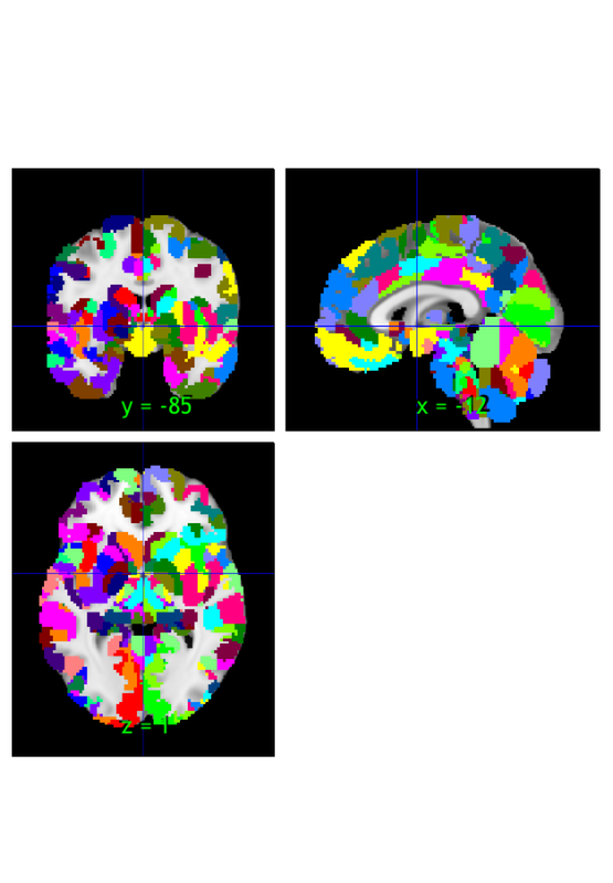
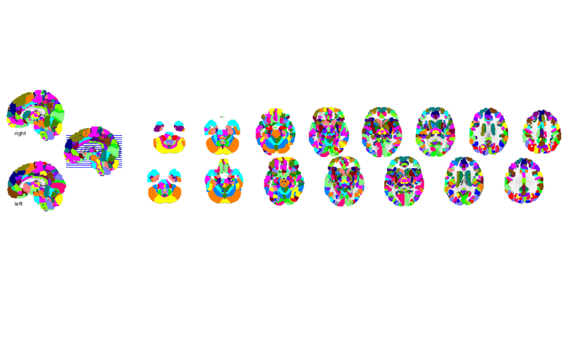
visualize the atlas regions
orthviews(atlas_obj);

o2 = montage(atlas_obj);

drawnow, snapnow
Grouping voxels with unique mask values, assuming integer-valued mask: 489 regions
select regions of interest
Let's select all the regions in the thalamus. All regions are labeled in the atlas object, so we can select them by name.
% Select all regions with "Thal" in the label:
thal = select_atlas_subset(atlas_obj, {'Thal'})

% Print the labels:
thal.labels

% Select a few thalamus/epithalamus regions of interest:
thal = select_atlas_subset(atlas_obj, {'Thal_Intra', 'Thal_VL', 'Thal_MD', 'Thal_LGN', 'Thal_MGN', 'Thal_Hb'});
thal.labels

% Select all the regions with "Thal" in the label, and collapse them into a single region:
whole_thal = select_atlas_subset(atlas_obj, {'Thal'}, 'flatten');
thal =

  atlas with properties:

               atlas_name: 'CANlab_2018_combined'
         probability_maps: [352328×17 double]
                   labels: {1×17 cell}
       label_descriptions: {17×1 cell}
                 labels_2: {1×17 cell}
                 labels_3: {1×17 cell}
                 labels_4: {''}
                 labels_5: {''}
               references: [33×485 char]
        space_description: 'MNI152 space'
    property_descriptions: {1×8 cell}
          additional_info: [0×0 struct]
                      dat: [352328×1 int32]
              dat_descrip: []
                  volInfo: [1×1 struct]
           removed_voxels: [352328×1 logical]
           removed_images: 0
              image_names: 'HCP-MMP1_on_MNI152_ICBM2009a_nlin.nii'
                 fullpath: '/Users/torwager/Documents/GitHub/Neuroimaging_Pattern_Masks/Atlases_and_parcellations/2018_Wager_combined_atlas/CANlab_2018_combined_atlas_2mm.nii'
              files_exist: 1
                  history: {1×5 cell}


ans =

  1×17 cell array

  Columns 1 through 4

    {'Thal_Pulv'}    {'Thal_LGN'}    {'Thal_MGN'}    {'Thal_VPL'}

  Columns 5 through 8

    {'Thal_VPM'}    {'Thal_Intralam'}    {'Thal_Midline'}    {'Thal_LD'}

  Columns 9 through 13

    {'Thal_VL'}    {'Thal_LP'}    {'Thal_VA'}    {'Thal_VM'}    {'Thal_MD'}

  Columns 14 through 17

    {'Thal_AM'}    {'Thal_AV'}    {'Thal_Hb'}    {'Thal_Hythal'}


ans =

  1×6 cell array

  Columns 1 through 4

    {'Thal_LGN'}    {'Thal_MGN'}    {'Thal_Intralam'}    {'Thal_VL'}

  Columns 5 through 6

    {'Thal_MD'}    {'Thal_Hb'}
load a dataset to extract data from for an ROI analysis
The dataset contains data from 33 participants, with brain responses to six levels of heat (non-painful and painful).
Aspects of this data appear in these papers: Wager, T.D., Atlas, L.T., Lindquist, M.A., Roy, M., Choong-Wan, W., Kross, E. (2013). An fMRI-Based Neurologic Signature of Physical Pain. The New England Journal of Medicine. 368:1388-1397 (Study 2)
Woo, C. -W., Roy, M., Buhle, J. T. & Wager, T. D. (2015). Distinct brain systems mediate the effects of nociceptive input and self-regulation on pain. PLOS Biology. 13(1): e1002036. doi:10.1371/journal.pbio.1002036
Lindquist, Martin A., Anjali Krishnan, Marina López-Solà, Marieke Jepma, Choong-Wan Woo, Leonie Koban, Mathieu Roy, et al. 2015. ?Group-Regularized Individual Prediction: Theory and Application to Pain.? NeuroImage. http://www.sciencedirect.com/science/article/pii/S1053811915009982.
This dataset is shared on figshare.com, under this link: https://figshare.com/s/ca23e5974a310c44ca93
Here is a direct link to the dataset file with the fmri_data object: https://ndownloader.figshare.com/files/12708989
The key variable is image_obj This is an fmri_data object from the CANlab Core Tools repository for neuroimaging data analysis. See https://canlab.github.io/
image_obj.dat contains brain data for each image (average across trials) image_obj.Y contains pain ratings (one average rating per image)
image_obj.additional_info.subject_id contains integers coding for which Load the data file, downloading from figshare if needed
Alternative sample datasets: -------------------------------------------- This dataset will take time to download from figshare if you haven't yet downloaded it. An alternative is to use the dataset included with the CANlab Core toolbox (though the results are less interesting for this example). image_obj = load_image_set('emotionreg');
A second example is a 270-person CANlab pain dataset shared on Neurovault. This is from Kragel et al. 2018, Nature Neuroscience. Try this to load it: test_images = load_image_set('kragel18_alldata', 'noverbose');
This uses the utility retrieve_neurovault_collection to pull the images from Neurovault.org if you don't have them. [files_on_disk, url_on_neurovault, mycollection, myimages] = retrieve_neurovault_collection(504); image_obj = fmri_data(files_on_disk);
fmri_data_file = which('bmrk3_6levels_pain_dataset.mat');

if isempty(fmri_data_file)

    % attempt to download
    disp('Did not find data locally...downloading data file from figshare.com')

    fmri_data_file = websave('bmrk3_6levels_pain_dataset.mat', 'https://ndownloader.figshare.com/files/12708989');

end

load(fmri_data_file);

descriptives(image_obj);
Source: BMRK3 dataset from CANlab, PI Tor Wager
Data: .dat contains 6 images per participant, activation estimates during heat on L arm from level 1(44.3 degrees C) to level 6(49.3), in 1 degree increments.


____________________________________________________________________________________________________________________________________________
 Wager, T.D., Atlas, L.T., Lindquist, M.A., Roy, M., Choong-Wan, W., Kross, E. (2013). An fMRI-Based Neurologic Signature of Physical Pain.
The New England Journal of Medicine. 368:1388-1397 (Study 2)

 Woo, C. -W., Roy, M., Buhle, J. T. & Wager, T. D. (2015). Distinct brain systems mediate the effects of nociceptive input and
self-regulation on pain. PLOS Biology. 13(1): e1002036. doi:10.1371/journal.pbio.1002036

Lindquist, Martin A., Anjali Krishnan, Marina López-Solà, Marieke Jepma, Choong-Wan Woo, Leonie Koban, Mathieu Roy, et al. 2015.
“Group-Regularized Individual Prediction: Theory and Application to Pain.” NeuroImage.
http://www.sciencedirect.com/science/article/pii/S1053811915009982.

____________________________________________________________________________________________________________________________________________

Summary of dataset
______________________________________________________
Images: 198	Nonempty: 198	Complete: 198
Voxels: 223707	Nonempty: 223707	Complete: 223707
Unique data values: 35583281

Min: -11.529	Max: 7.862	Mean: -0.004	Std: 0.227

    Percentiles      Values
    ___________    __________

        0.1            -1.529
        0.5          -0.88055
          1          -0.67632
          5          -0.31891
         25         -0.087519
         50        0.00034864
         75          0.087461
         95           0.29757
         99           0.60449
       99.5           0.77676
       99.9            1.3177
extract data from each atlas region
- "r" is a region-class object. see >> help region - r(i).dat contains averages over voxels within region i. for n images, it contains an n x 1 vector with average data. - r(i).data contains an images x voxels matrix of all data within region i.
r = extract_roi_averages(image_obj, thal);
fmri_data.extract_roi_averages: Defining mask object. Resampling mask.
Grouping voxels with unique mask values, assuming integer-valued mask:   6 regions
Averaging data. Averaging over unique mask values, assuming integer-valued mask:   6 regions
Done.
You could also extract data from the whole thalamus into a single variable using: r = extract_roi_averages(data_obj, whole_thal);
An alternative is the extract_data method: region_avgs = extract_data(thal, image_obj); The values may differ slightly based on which image is being resampled to which. Resampling matches the voxels in two sets of images that may have different voxel sizes and voxel boundaries by interpolating values from one to match the space of the other.
Do a group ROI analysis and make a "violin plot" (or barplot) for each region
We'll use the barplot_columns function, which is a versatile function for plotting columns of matrices. It has many options for displaying or hiding individual data points, "violins" (distribution estimates), standard errors, and more.
The barplot_columns function also does a basic one-sample t-test analysis on each column, which corresponds to the average of each region here. This ROI analysis can be used for inference about a region.
With the pain dataset, for a real analysis we might worry that multiple images come from the same subject. We can't do stats across all the iamges without accounting for the correlations among images belonging to the same subject. But first, let's plot the averages and see waht we get:
% Concatenate the region averages into a matrix:
roi_averages = cat(2, r.dat);

% Get the labels for each region from the atlas object, \
% and replace some characters to make them look a bit nicer:
thal_labels = format_strings_for_legend(thal.labels);

% Now make the figure:
create_figure('Thalamus regions', 1, 2);

barplot_columns(roi_averages, 'nofig', 'colors', scn_standard_colors(length(r)), 'names', thal_labels);
xlabel('Region')
ylabel('ROI activity')

subplot(1, 2, 2)

barplot_columns(roi_averages, 'nofig', 'colors', scn_standard_colors(length(r)), 'names', thal_labels, 'noind', 'noviolin');
xlabel('Region')
ylabel('ROI activity')
Col   1: Thal LGN	Col   2: Thal MGN	Col   3: Thal Intralam	Col   4: Thal VL	Col   5: Thal MD	Col   6: Thal Hb
---------------------------------------------
Tests of column means against zero
---------------------------------------------
         Name          Mean_Value    Std_Error      T           P         Cohens_d
    _______________    __________    _________    ______    __________    ________

    'Thal LGN'         -0.012699      0.004484    -2.832     0.0051061    -0.20126
    'Thal MGN'          0.010652     0.0057635    1.8481      0.066087     0.13134
    'Thal Intralam'      0.03687       0.00871    4.2331    3.5331e-05     0.30083
    'Thal VL'           0.041771     0.0066064    6.3229    1.6843e-09     0.44935
    'Thal MD'           0.041843      0.012939    3.2338     0.0014324     0.22982
    'Thal Hb'           0.027095       0.01771    1.5299       0.12764     0.10873
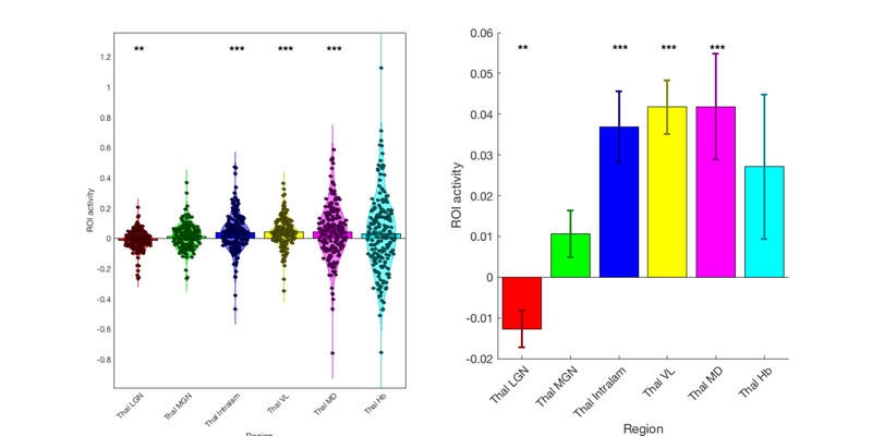
Look at the results. Do they make sense for a pain dataset? The sensory/nociceptive regions of the thalamus (VL and intralaminar) respond to painful stimuli, but not the regions in visual and auditory pathways (LGN, MGN). The habenula also responds.
To do a proper ROI analysis, let's just select a subset of the images responding to one stimulus intensity, with one image per person. the stimulus temperatures are stored in image_obj.additional_info.temperatures So we can use basic Matlab code to select one temperature.
wh = image_obj.additional_info.temperatures == 48;  % A logical vector for 48 degrees
indx_list = find(wh);                               % a list of which images

image_obj_48 = get_wh_image(image_obj, indx_list);  % Get the images we want

% You can try to extract data from the thalamus and repeat the t-test.
Explore on your own
1. One of the ideas about emotion regulation is that positive appraisal involves activity increases in the nucleus accumbens (NaC) in the basal ganglia. Load the emotion regulation dataset from previous walkthroughs. Try to locate and extract data from this region, and do an ROI analysis. What do you see?
2. try the t-test on 48 degree only images above. What do you see? Which regions show sigificant activation?
3. Try to identify which prefrontal regions show the greatest emotion regulation effect, and which show the greatest response during pain. Are they the same?
% That's it for this section!!