Contents
Applying masks and writing image data to disk
% One common operation in neuroimaging is masking. Masking is defining a set
% of voxels to include or exclude from analysis or presentation. Some uses
% include:
%
% * Apply a generous brain mask to store only in-brain voxels, saving space,
%   (CANlab data objects do this by default, with a liberal mask)
% * Identify gray matter voxels to calculate global mean signal or other metrics
% * Identify voxels in ventricles or out-of-brain to try to isolate sources
%   of noise or artifacts to remove
% * Identify gray matter voxels of interest to limit the space within which
%   you correct for multiple comparisons, thus increasing power
% * Limiting presentation of results to an a priori set of ROIs
% * Limiting the scope of training or testing a multivariate pattern or
%   predictive model, to help test hypotheses about which systems/regions
%   contribute to prediction.
%
The Neuroimaging_pattern_masks Github repository and website
For this walkthrough, we'll load some new image datasets to use as masks. A popular one is a set of "networks" developed from resting-state fMRI connectivity in 1,000 people. For our purposes, the "network" maps consist of a set of voxels that load most highly on each of 7 ICA components from the 1,000 Functional Connectomes project. These were published by Randy Buckner's lab in 2011 in three papers: Choi et al., Buckner et al., and Yeo et al. We'll use the cortical networks from Yeo et al. here.
This set of images and other broadly useful sets of images are stored in the CANlab function load_image_set in a registry that you can access by name. Try help load_image|set for a list of images you can load by keyword. These datasets, if they can be stored on Github, are in this Github repository:
https://github.com/canlab/Neuroimaging_Pattern_Masks
In addition, you can explore these and find more information here: https://sites.google.com/dartmouth.edu/canlab-brainpatterns/home
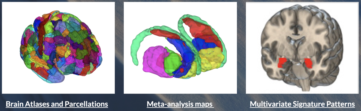
To run this tutorial and many others in this series, you'll need to download the Neuroimaging_Pattern_Masks Github repository and add it to your Matlab path with subfolders. The Github site has three main types of datasets, shown here:
Load and select a sample mask
You will need the Neuroimaging_Pattern_Masks repository installed to find these images.
[bucknermaps, mapnames] = load_image_set('bucknerlab'); % loads 7 masks from Yeo et al.
Loaded images:
/Users/torwager/Documents/GitHub/CanlabCore/CanlabCore/canlab_canonical_brains/Combined_multiatlas_ROI_masks/rBucknerlab_7clusters_SPMAnat_Other_combined.img
This loads 7 images. try orthviews(dat) to see them all. What values do the images have? You can also see descriptive statistics for the images like this:
desc = descriptives(bucknermaps);
Source: Info about image source here


Summary of dataset
______________________________________________________
Images:   7	Nonempty:   7	Complete:   7
Voxels: 352328	Nonempty: 131918	Complete:   0
Unique data values:   1

Min: 1.000	Max: 1.000	Mean: 1.000	Std: 0.000

    Percentiles    Values
    ___________    ______

        0.1          1
        0.5          1
          1          1
          5          1
         25          1
         50          1
         75          1
         95          1
         99          1
       99.5          1
       99.9          1
The variable desc is a structure that contains various descriptive stats.
load_image_set will generally store and return names for each image, returned as outputs if requested (here in mapnames). Let's print those names:
disp(char(mapnames))
Visual
Somatomotor
dAttention
vAttention
Limbic
Frontoparietal
Default
Now we can select one image from those 7 to use as a mask.
mask_image = bucknermaps.get_wh_image(1);
Now we'll load a sample dataset to apply the mask to. This loads a series of 7 muoltivariate patterns from Kragel et al. 2016. These patterns were developed to predict emotion categories. For our purposes here, we'll just treat them as data images.
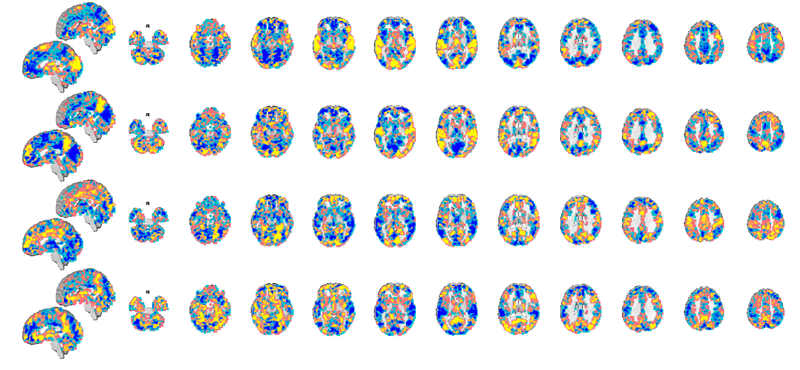
test_dat = load_image_set('kragelemotion', 'noverbose'); % loads 7 masks from Kragel et al.

% Try |orthviews(dat)| or use |montage| to see these patterns.
% This command shows the first 4 (a limit in |montage| to avoid messy
% displays):

montage(test_dat);
Warning: Showing first 4 images in data object only.
Setting up fmridisplay objects
This takes a lot of memory, and can hang if you have too little.
Grouping contiguous voxels:   8 regions
sagittal montage: 1329 voxels displayed, 17999 not displayed on these slices
axial montage: 7967 voxels displayed, 11361 not displayed on these slices
Grouping contiguous voxels:   8 regions
sagittal montage: 1329 voxels displayed, 17999 not displayed on these slices
axial montage: 7967 voxels displayed, 11361 not displayed on these slices
Grouping contiguous voxels:   8 regions
sagittal montage: 1329 voxels displayed, 17999 not displayed on these slices
axial montage: 7967 voxels displayed, 11361 not displayed on these slices
Grouping contiguous voxels:   8 regions
sagittal montage: 1329 voxels displayed, 17999 not displayed on these slices
axial montage: 7967 voxels displayed, 11361 not displayed on these slices
Apply a mask
We can apply the mask using the apply_mask() method for fmri_data objects. It has various options, but the simplest one applies a single mask to an fmri_data object. As a rule, you should pass in the object you're operating on first, followed by additional modifying arguments/objects. Here, this means data object followed by mask object.
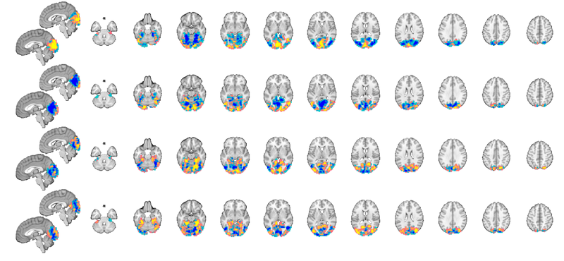
test_dat = apply_mask(test_dat, mask_image);

% Now let's view the new, masked dataset:

montage(test_dat);

% Now, the dataset contains only voxels in the "visual network", and
% subsequent analyses or operations would test only that.
Warning: Showing first 4 images in data object only.
Setting up fmridisplay objects
This takes a lot of memory, and can hang if you have too little.
Grouping contiguous voxels:   2 regions
sagittal montage: 201 voxels displayed, 3097 not displayed on these slices
axial montage: 1647 voxels displayed, 1651 not displayed on these slices
Grouping contiguous voxels:   2 regions
sagittal montage: 201 voxels displayed, 3097 not displayed on these slices
axial montage: 1647 voxels displayed, 1651 not displayed on these slices
Grouping contiguous voxels:   2 regions
sagittal montage: 201 voxels displayed, 3097 not displayed on these slices
axial montage: 1647 voxels displayed, 1651 not displayed on these slices
Grouping contiguous voxels:   2 regions
sagittal montage: 201 voxels displayed, 3097 not displayed on these slices
axial montage: 1647 voxels displayed, 1651 not displayed on these slices
A few exercises
1. Here's a question to answer: What are some potential uses of the masking operation we did above? Why would you want to do it?
2. Try loading the emotion regulation dataset from previous tutorials, and do a one-sample t-test group analysis only within the "frontoparietal" network. Try thresholding the results with FDR correction for both the full dataset and the analysis within the restricted mask. How are the results different? Why?
Writing image data in objects to Nifti files on disk
canlabcore fmri data objects can be easily written to standard image file formats. The main function for this is write()
This walkthrough shows how to do this for 1) a mask image, and 2) a statistic image.
Create a Nifti image called dummy.nii in the current folder. Write the mask image to this file. See help for write() for more options
fname = 'dummy.nii';  % outname file name.  the extension (.nii, .img) determines the format.

% |write(mask_image, 'fname', fname);|
If you've already done this, write() will return an error. This is a safeguard to keep users from inadvertently overwriting important files. To force overwriting the existing file, try:
write(mask_image, 'fname', fname, 'overwrite');
Writing:
dummy.nii
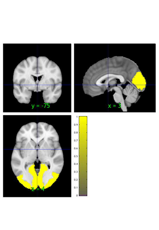
Now let's read it back in from disk and view it again:
orthviews(fmri_data(fname))
Using default mask: /Users/torwager/Documents/GitHub/CanlabCore/CanlabCore/canlab_canonical_brains/Canonical_brains_surfaces/brainmask.nii
loading mask. mapping volumes.
checking that dimensions and voxel sizes of volumes are the same.
Pre-allocating data array. Needed: 1409312 bytes
Loading image number:     1
Elapsed time is 0.022505 seconds.
Image names entered, but fullpath attribute is empty. Getting path info.
Grouping contiguous voxels:   3 regions

ans =

  1×1 cell array

    {1×3 region}
Exercises
1. Select a sample image from test_dat, threshold it at an arbitrary threshold of absolute values > .0005, and write it to disk. Load it again from disk and display it. See the thresholding walkthrough for more help if needed.
2. Do the one-sample t-test on the emotion regulation dataset (see the t-test walkthrough if needed), and threshold the results at 0.05 FDR-corrected. Write the thresholded results map to disk. Reload it from disk and display it using the montage() method.