3-D volume visualization
Contents
- About volume visualisation
- Prepare sample statistical results maps
- The surface() method
- Using MNISurf volume to surface projection
- Using the fmridisplay object to create a registry of montages/surfaces
- Using addbrain to load or build surfaces
- Removing blobs and re-adding new colors
- Prepackaged cutaway surfaces
- Creating isosurfaces
- Using isosurface to create a custom surface
- Explore on your own
- Explore More: CANlab Toolboxes
About volume visualisation
Creating 3-D renderings of brain data and results can help localize brain activity and show patterns in a way that allows meaningful comparisons across studies.
The CANlab object-oriented tools have methods built in for rendering volume data on brain surfaces. They generally use Matlab's isosurface and isocaps functions. These tools can (optionally) incorporate information about source volumetric templates and target surface templates to more accurately render surface plots, and the use of these features is highly recommended. If enabled, MNISurf projection is used, as detailed by Wu et al. (2018) Human Brain Mapping.
Prepare sample statistical results maps
For this walkthrough, we'll use the "Pain, Cognition, Emotion balanced N = 270 dataset" from Kragel et al. 2018, Nature Neuroscience. More information about this dataset and how to download it is in an earlier walkthrough on "loading datasets"
The code below loads it; but you could also use any other brain dataset for this purpose (e.g., the 'emotionreg' dataset in load_image_set.
Our goal is to select subject-level images corresponding to a particular task type and do a t-test on these, and visualize the results in various 3-D ways.
[test_images, names] = load_image_set('kragel18_alldata', 'noverbose');

% This field contains a table object with metadata for each image:

metadata = test_images.metadata_table;
metadata(1:5, :)                        % Show the first 5 rows

% Here are the 3 domains:

disp(unique(metadata.Domain))

% Find all the images of "Neg_Emotion" and pull those into a separate
% fmri_data object:

wh = find(strcmp(metadata.Domain, 'Neg_Emotion'));
neg_emo = get_wh_image(test_images, wh);

% Do a t-test on these images, and store the results in a statistic_image
% object called "t". Threshold at q < 0.001 FDR. This is an unusual
% threshold, but we have lots of power here, and want to restrict the
% number of significant voxels for display purposes below.

t = ttest(neg_emo, .001, 'fdr');

% Find the images for other conditions and save them for later:

t_emo = t;

wh = find(strcmp(metadata.Domain, 'Cog_control'));
cog_control = get_wh_image(test_images, wh);
t_cog = ttest(cog_control, .001, 'fdr');

wh = find(strcmp(metadata.Domain, 'Pain'));
pain = get_wh_image(test_images, wh);
t_pain = ttest(pain, .001, 'fdr');
Loading /home/bogdan/.matlab/canlab/CANlab_help_examples/example_help_files/kragel_2018_nat_neurosci_270_subjects_test_images.mat

ans =

  5×6 table

     Domain      Subdomain        imagenames       Studynumber    Orig_Studynumber        StudyCodes
    ________    ___________    ________________    ___________    ________________    __________________

    {'Pain'}    {'Thermal'}    {'ThermalPain1'}         1                10           {'Atlas_2010_EXP'}
    {'Pain'}    {'Thermal'}    {'ThermalPain1'}         1                10           {'Atlas_2010_EXP'}
    {'Pain'}    {'Thermal'}    {'ThermalPain1'}         1                10           {'Atlas_2010_EXP'}
    {'Pain'}    {'Thermal'}    {'ThermalPain1'}         1                10           {'Atlas_2010_EXP'}
    {'Pain'}    {'Thermal'}    {'ThermalPain1'}         1                10           {'Atlas_2010_EXP'}

    {'Cog_control'}
    {'Neg_Emotion'}
    {'Pain'       }

One-sample t-test
Calculating t-statistics and p-values
Image   1 FDR q < 0.001 threshold is 0.000115

Image   1
 92 contig. clusters, sizes   1 to 12460
Positive effect: 20246 voxels, min p-value: 0.00000000
Negative effect: 2957 voxels, min p-value: 0.00000000
One-sample t-test
Calculating t-statistics and p-values
Image   1 FDR q < 0.001 threshold is 0.000000

Image   1
  0 contig. clusters, sizes     to
Positive effect:   0 voxels, min p-value: 0.00000048
Negative effect:   0 voxels, min p-value: 0.00001979
One-sample t-test
Calculating t-statistics and p-values
Image   1 FDR q < 0.001 threshold is 0.000057

Image   1
 97 contig. clusters, sizes   1 to 3560
Positive effect: 7006 voxels, min p-value: 0.00000000
Negative effect: 4481 voxels, min p-value: 0.00000000
The surface() method
Most data objects, including fmri_data, statistic_image, and region objects, have a surface() method. Entering it with no arguments creates a surface or series of surfaces (depending on the object)
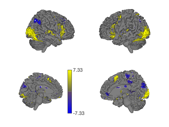
The surface() method lets you easily render blobs on a number of pre-set choices for brain surfaces or 3-D cutaway surfaces.
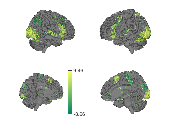
% This generates a series of 6 surfaces of different types, including a
% subcortical cutaway

surface(t);
drawnow, snapnow

% This generates a different plot

create_figure('lateral surfaces');
surface_handles = surface(t, 'foursurfaces', 'noverbose');
snapnow

% You can see more options with:
% |help statistic_image.surface| or |help t.surface|

% You can also use the |render_on_surface()| to method to change the colormap:

render_on_surface(t, surface_handles, 'colormap', 'summer');
snapnow
Anatomical image: Adapted from the 7T high-resolution atlas of Keuken, Forstmann et al.
Keuken et al. (2014). Quantifying inter-individual anatomical variability in the subcortex using 7T structural MRI.
Forstmann, Birte U., Max C. Keuken, Andreas Schafer, Pierre-Louis Bazin, Anneke Alkemade, and Robert Turner. 2014. ?Multi-Modal Ultra-High Resolution Structural 7-Tesla MRI Data Repository.? Scientific Data 1 (December): 140050.
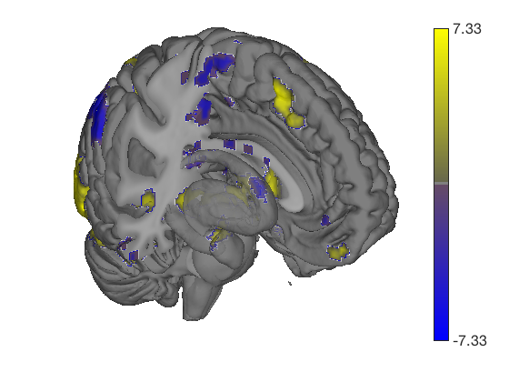
Using MNISurf volume to surface projection
The above plots are rendered by cross referencing the coordinates of voxels in MNI space with the coordinates of vertices in a brain surface object, "BigBrain" in this case. These vertices of corresponding anatomy does not in general coincide across these volume and surface formats. For instance, the coordinates of the cortical gray matter mantel in a brain registered to the MNI152NLin2009cAsym volumetric template may fall at a greater radial distance from the center of the brain than the cortical mantel in bigbrain or vice versa resulting incorrect rendering of deep cortical signals from the volumetric data to superficial locations in the surface template.
To address this issue we've run segmentations of MNI templates using freesurfer to obtain template specific cortical surfaces. These template specific surfaces were then registered and resampled to a couple surface templates, initially HCP's fsLR 32k and freesurfer's fsaverage 164k, although more may be added in the future. These are then used to establish voxel-to-surface interpolation maps which will generalize to a particular surface (e.g. HCP's fsLR 32k) at any particular level of inflation from uninflated to flat maps. In order to take advantage of this functionality you simply need to specify the source space (a MNI template) and a target surface (fsLR_32k or fsaverage164k)
% Here is an example of the above data projected to the inflated fsLR 32k
% surface used by HCP grayordinate formats.

create_figure('lateral surfaces');
surface_handles = surface(t, 'hcp inflated left')

% Here is an example of the same data remapped with source and target
% awareness
create_figure('lateral surfaces');
surface_handles = surface(t, 'hcp inflated left', 'sourcespace', 'MNI152NLin2009cAsym', 'targetsurface', 'fsLR_32k')

% Although we do not in this case know precisely which sourcespace to use
% (the kragel dataset is a multistudy aggregate that likely was registered
% to multiple different MNI templates), you can still see what an impact
% using MNISurf projection can have. Notably, there is no MNISurf
% projection for the bigbrain surfaces. In some cases, the targetsurface
% may be detected automatically (e.g. if using canlab_results_fmridisplay()
% presets), and can be ommitted, but if needed you will be prompted by a
% warning and available options are enumerated. However, you must always
% specify a sourcespace manually so pay attention to what templates your
% volumetric data are registered too to be able to use this functionality
% correctly.
surface_handles =

  Patch (hcp inflated left) with properties:

    FaceColor: 'interp'
    FaceAlpha: 1
    EdgeColor: 'none'
    LineStyle: '-'
        Faces: [64980×3 int32]
     Vertices: [32492×3 single]

  Use GET to show all properties

Warning: Unknown input string option:MNI152NLin2009cAsym
Warning: Unknown input string option:targetsurface
Warning: Unknown input string option:fsLR_32k

surface_handles =

  Patch (hcp inflated left) with properties:

    FaceColor: 'interp'
    FaceAlpha: 1
    EdgeColor: 'none'
    LineStyle: '-'
        Faces: [64980×3 int32]
     Vertices: [32492×3 single]

  Use GET to show all properties
Using the fmridisplay object to create a registry of montages/surfaces
The fmridisplay object is an object class that stores information about a set of display items you have created. It stores information about a series of montages (in the same figure or different figures) and surfaces along with their handles.
You can use this to render activations on a whole set of slices/surfaces at once. You can create your own custom views, or use pre-packaged sets of montages/surfaces created by the function canlab_results_fmridisplay
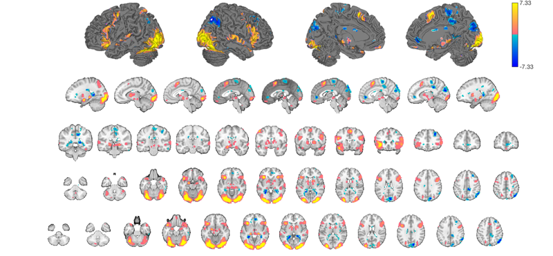
The code snippet below displays our t-map on a relatively complete series of slices and surfaces, so you can see the "whole picture".
my_display_obj = canlab_results_fmridisplay([], 'montagetype', 'full');
my_display_obj = addblobs(my_display_obj, region(t));
snapnow
Setting up fmridisplay objects
Compressed NIfTI files are not supported.
    48

Grouping contiguous voxels:  92 regions
sagittal montage: 2999 voxels displayed, 20204 not displayed on these slices
coronal montage: 2250 voxels displayed, 20953 not displayed on these slices
axial montage: 5579 voxels displayed, 17624 not displayed on these slices
axial montage: 5517 voxels displayed, 17686 not displayed on these slices
You can see some prepackaged sets in help canlab_results_fmridisplay These include: 'full' Axial, coronal, and saggital slices, 4 cortical surfaces 'compact' Midline saggital and two rows of axial slices [the default] 'compact2' A single row showing midline saggital and axial slices 'multirow' A series of 'compact2' displays in one figure for comparing different images/maps side by side 'regioncenters' A series of separate axes, each focused on one region
In addition, you can pass in a series of optional keywords that will be passed onto the addblobs object method that controls rendering of the blobs on slices. (They don't all work for surfaces). These control colors, inclusion of an outline around each activation blob/region, and more. See help fmridisplay.addblobs for more information. Here is an example using a few of the options.
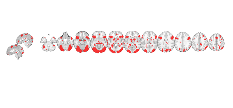
my_display_obj = canlab_results_fmridisplay(t, 'compact2', 'color', [1 0 0], 'nooutline', 'trans');
Grouping contiguous voxels:  92 regions
Setting up fmridisplay objects
Compressed NIfTI files are not supported.
axial montage: 5570 voxels displayed, 17633 not displayed on these slices
sagittal montage: 427 voxels displayed, 22776 not displayed on these slices
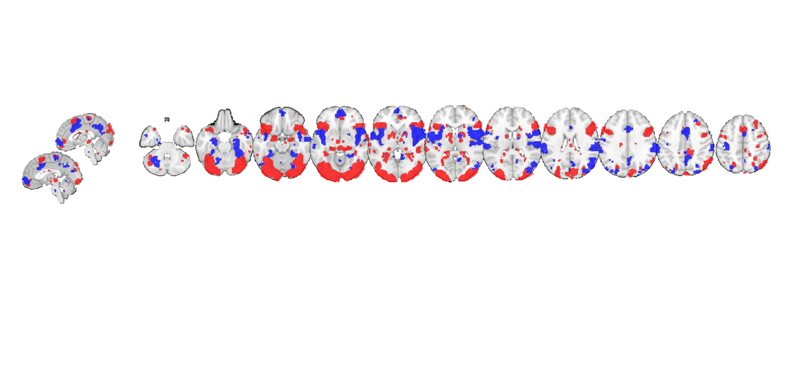
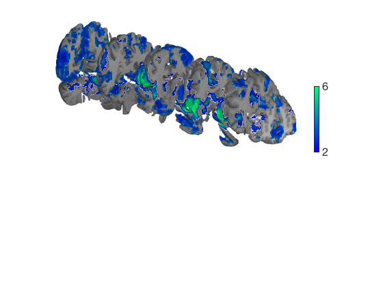
After creating the display, other maps can be added. The addblobs() method requires a region object, so we use region(t) to convert to a region object. This shows us regions activated during negative emotion in red and pain in blue.
my_display_obj = addblobs(my_display_obj, region(t_pain), 'color', [0 0 1], 'nooutline', 'trans');
snapnow
Grouping contiguous voxels:  97 regions
axial montage: 2814 voxels displayed, 8673 not displayed on these slices
sagittal montage: 495 voxels displayed, 10992 not displayed on these slices
my_display_obj is an fmridisplay-class object. It has its own methods:
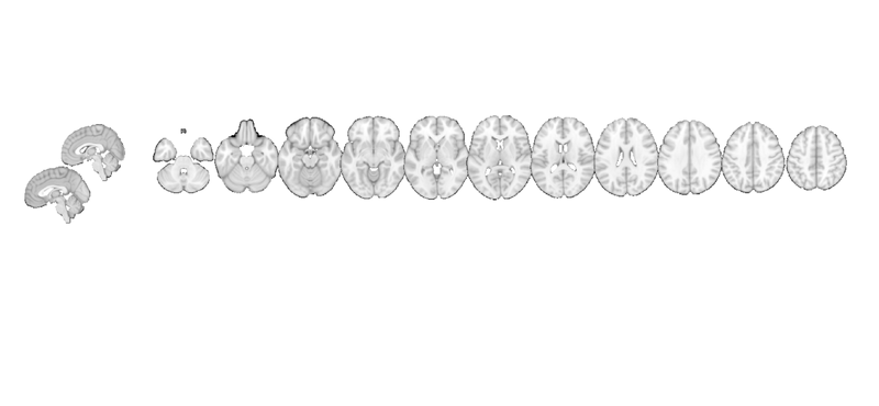
methods(my_display_obj)

% One particularly useful feature is that you can add or _remove_ activation blobs.
% This allows you to create a canonical set of views and then render one
% activation map on them, remove the blobs, and render other maps on the
% same set of display items. You can add points, spheres (e.g., from
% different studies), and more.
%
% When you operate on an fmridisplay object, pass it back out as an output
% argument so that the information you updated will be available.

my_display_obj = removeblobs(my_display_obj);
snapnow
Methods for class fmridisplay:

activate_figures     legend               title_montage
addblobs             montage              transparency_change
addpoints            removeblobs          zoom_in_on_regions
addthreshblobs       removepoints
fmridisplay          surface
Using addbrain to load or build surfaces
You can also build any surface object you want and render colors onto it. This is a very versatile method.
Matlab creates handles to surfaces (and other graphics objects). You can use the handles to manipulate the objects in a many ways. They have, for example, color, line, face color, edge color, and many more properties. If h is a figure handle, get(h) shows a list of its properties. set(h, 'MyPropertyName', myvalue) sets the property 'MyPropertyName' to myvalue.
Here, we'll use addbrain to build up a set of surfaces with handles, and then render colored blobs on them using surface(). Instead of the object method, you can also use its underlying function: cluster_surf
Try help addbrain for a list of surfaces, and help cluster_surf for other color/display/scaling options.
Note: this step requires access to the MasksPrivate repo
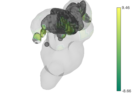
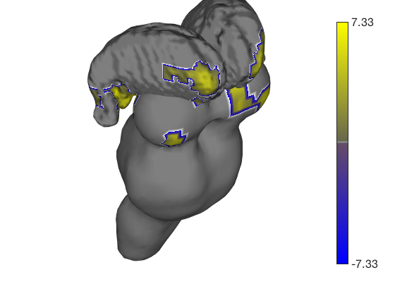
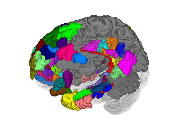
% Let's build a surface by starting with a group of thalamic nuclei, and
% adding the parabrachial complex and the red nucleus.
% Then, we'll render our t-statistics in colors onto those surfaces.

create_figure('cutaways'); axis off
surface_handles = addbrain('thalamus_group');

surface_handles = [surface_handles addbrain('pbn')];
surface_handles = [surface_handles addbrain('rn')];
surface_handles = [surface_handles addbrain('pag')];

drawnow, snapnow
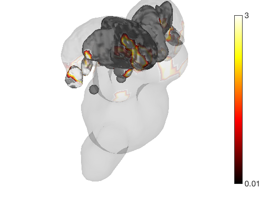
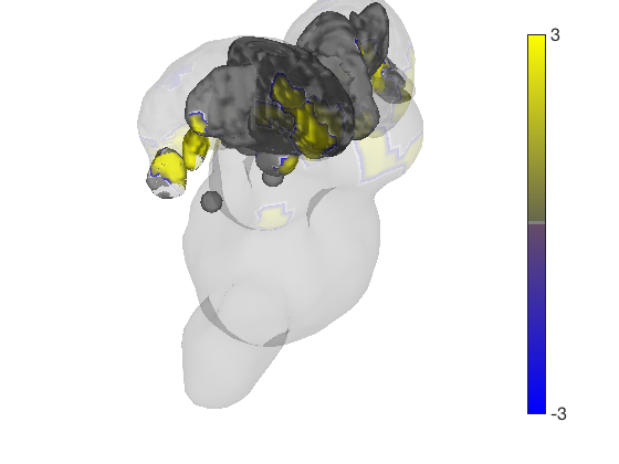
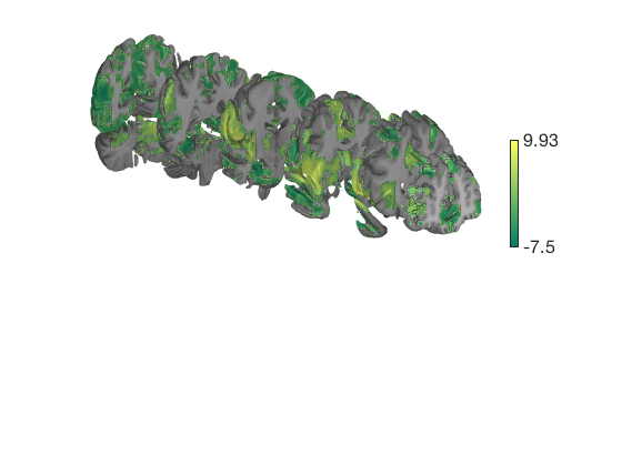
Now render the statistic image stored in t onto those surfaces. All non-activated areas turn gray.
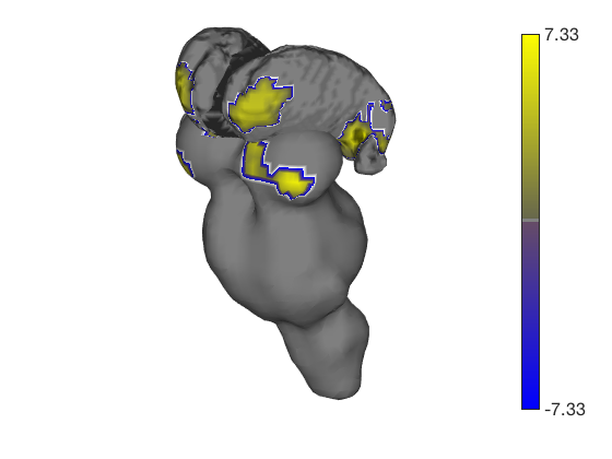
render_on_surface(t, surface_handles, 'colormap', 'summer');
set(surface_handles, 'FaceAlpha', .85);
set(surface_handles(5:6), 'FaceAlpha', .15);   % Make brainstem and thalamus shell more transparent
drawnow, snapnow

% Emphasize positive values, in a hot colormap
render_on_surface(t, surface_handles, 'clim', [0.01 3]);
drawnow, snapnow

% Show positive and negative values, in a hot colormap
render_on_surface(t, surface_handles, 'clim', [-3 3]);
drawnow, snapnow
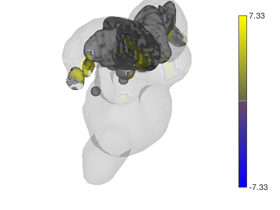
Now render the statistic image stored in t onto those surfaces. All non-activated areas turn gray.
t.surface('surface_handles', surface_handles, 'noverbose');
drawnow, snapnow
Transparent surfaces are a little hard to see. We can use Matlab's powerful handle graphics system to inspect and change all kinds of properties. See the Matlab documentation for more details. Let's just make the surfaces solid:
set(surface_handles, 'FaceAlpha', 1);
drawnow, snapnow
These surfaces can be rotated too (or zoom in/out, pan, set lighting, etc.) Let's shift the angle.
axes(get(surface_handles(1),'Parent'));

view(222, 15);          % rotate
camzoom(0.8);           % zoom out

% A helpful CANlab function to re-set the lighting after rotating is:

lightRestoreSingle;

drawnow, snapnow
addbrain also has keywords for composites of multiple surfaces
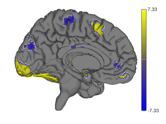
create_figure('cutaways'); axis off
surface_handles = addbrain('limbic');
ax = gca
ax.Position(1) = ax.Position(1) - 0.1; % to avoid colorbar overlap
t.surface('surface_handles', surface_handles, 'noverbose');
ax =

  Axes with properties:

             XLim: [-71.3413 36.6702]
             YLim: [-106.2400 73.8421]
           XScale: 'linear'
           YScale: 'linear'
    GridLineStyle: '-'
         Position: [0.1300 0.1100 0.7750 0.8150]
            Units: 'normalized'

  Use GET to show all properties
Removing blobs and re-adding new colors
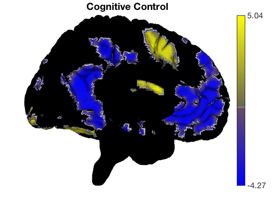
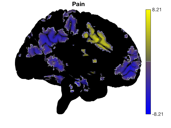
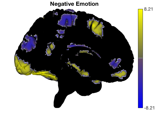
There is a special command to re-set the surface colors to gray. Then we can add a t-test for different contrasts without re-drawing surfaces.
surface_handles = addbrain('eraseblobs',surface_handles);

title('Cognitive Control');
t = ttest(cog_control, .001, 'unc');
t.surface('surface_handles', surface_handles, 'noverbose');
drawnow, snapnow

surface_handles = addbrain('eraseblobs',surface_handles);

title('Pain');
t = ttest(pain, .001, 'unc');
t.surface('surface_handles', surface_handles, 'noverbose');
drawnow, snapnow

surface_handles = addbrain('eraseblobs',surface_handles);

title('Negative Emotion');
t = ttest(neg_emo, .001, 'unc');
t.surface('surface_handles', surface_handles, 'noverbose');
drawnow, snapnow
One-sample t-test
Calculating t-statistics and p-values

Image   1
 62 contig. clusters, sizes   1 to 3466
Positive effect: 9738 voxels, min p-value: 0.00000048
Negative effect: 12395 voxels, min p-value: 0.00001979
One-sample t-test
Calculating t-statistics and p-values

Image   1
162 contig. clusters, sizes   1 to 4676
Positive effect: 11179 voxels, min p-value: 0.00000000
Negative effect: 13188 voxels, min p-value: 0.00000000
One-sample t-test
Calculating t-statistics and p-values

Image   1
 95 contig. clusters, sizes   1 to 15543
Positive effect: 30474 voxels, min p-value: 0.00000000
Negative effect: 6758 voxels, min p-value: 0.00000000
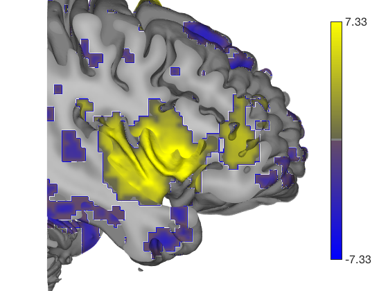
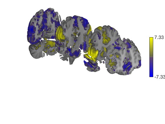
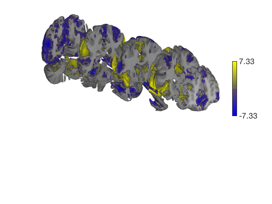
Prepackaged cutaway surfaces
Addbrain has many 3-D surfaces, including cutaways that show various 3-D sections. The code below visualizes the various options for cutaways.
You can also pass any of these keywords into surface() to generate the surface and render colored blobs. Let's render these with and without an unthresholded pain map
t = ttest(pain, 1, 'unc');
t_thr = threshold(t, .05, 'fdr');

keywords = {'left_cutaway' 'right_cutaway' 'left_insula_slab' 'right_insula_slab' 'accumbens_slab' 'coronal_slabs' 'coronal_slabs_4' 'coronal_slabs_5'};

for i = 1:length(keywords)

    create_figure('cutaways'); axis off

    surface_handles = surface(t_thr, keywords{i});

    % This essentially runs the code below:

    % surface_handles = addbrain(keywords{i}, 'noverbose');
    % render_on_surface(t, surface_handles, 'clim', [-7 7]);

    % Alternative: This command creates the same surfaces:
    % surface_handles = canlab_canonical_brain_surface_cutaways(keywords{i});
    % render_on_surface(t, surface_handles, 'clim', [-7 7]);

    drawnow, snapnow

end
One-sample t-test
Calculating t-statistics and p-values

Image   1
 17 contig. clusters, sizes   1 to 201248
Positive effect: 75756 voxels, min p-value: 0.00000000
Negative effect: 125519 voxels, min p-value: 0.00000000
Image   1 FDR q < 0.050 threshold is 0.012390

Image   1
231 contig. clusters, sizes   1 to 26709
Positive effect: 17979 voxels, min p-value: 0.00000000
Negative effect: 31899 voxels, min p-value: 0.00000000
Anatomical image: Adapted from the 7T high-resolution atlas of Keuken, Forstmann et al.
Keuken et al. (2014). Quantifying inter-individual anatomical variability in the subcortex using 7T structural MRI.
Forstmann, Birte U., Max C. Keuken, Andreas Schafer, Pierre-Louis Bazin, Anneke Alkemade, and Robert Turner. 2014. ?Multi-Modal Ultra-High Resolution Structural 7-Tesla MRI Data Repository.? Scientific Data 1 (December): 140050.
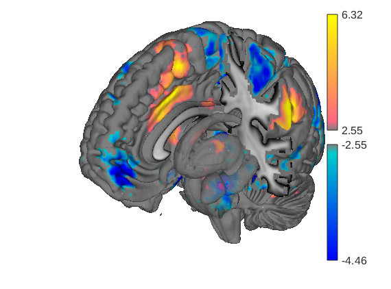
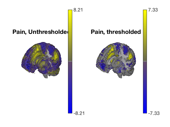
Plot thresholded and unthresholded maps side by side
create_figure('cutaways',1, 2); axis off

surface_handles = surface(t, 'right_cutaway');
title('Pain, Unthresholded')

subplot(1, 2, 2);
surface_handles = surface(t_thr, 'right_cutaway');
title('Pain, thresholded')

drawnow, snapnow
Anatomical image: Adapted from the 7T high-resolution atlas of Keuken, Forstmann et al.
Keuken et al. (2014). Quantifying inter-individual anatomical variability in the subcortex using 7T structural MRI.
Forstmann, Birte U., Max C. Keuken, Andreas Schafer, Pierre-Louis Bazin, Anneke Alkemade, and Robert Turner. 2014. ?Multi-Modal Ultra-High Resolution Structural 7-Tesla MRI Data Repository.? Scientific Data 1 (December): 140050.
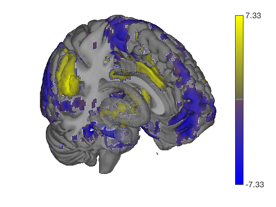
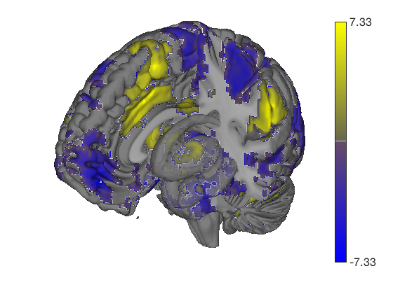
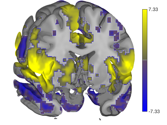
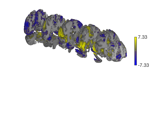
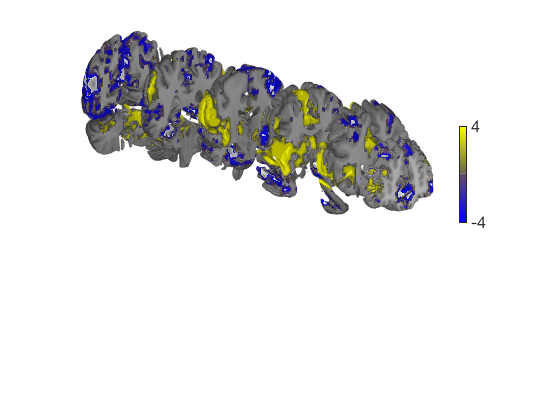
Controlling options in render_on_surface()
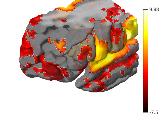
When the t map has positive and negative values, render_on_surface creates a special bicolor split colormap that has warm colors for positive vals, and cool colors for negative vals. You can set the color limits (here, in t-values)
create_figure('cutaways'); axis off
surface_handles = surface(t_thr, 'coronal_slabs');

render_on_surface(t_thr, surface_handles, 'clim', [-4 4]);
drawnow, snapnow

% You can set the colormap to any Matlab colormap:
render_on_surface(t_thr, surface_handles, 'colormap', 'summer');
drawnow, snapnow

% If your image is positive-valued only (or negative-valued only), a
% bicolor split map will not be created:

t = threshold(t_thr, [2 Inf], 'raw-between');
surface_handles = surface(t, 'coronal_slabs');
drawnow, snapnow
Anatomical image: Adapted from the 7T high-resolution atlas of Keuken, Forstmann et al.
Keuken et al. (2014). Quantifying inter-individual anatomical variability in the subcortex using 7T structural MRI.
Forstmann, Birte U., Max C. Keuken, Andreas Schafer, Pierre-Louis Bazin, Anneke Alkemade, and Robert Turner. 2014. ?Multi-Modal Ultra-High Resolution Structural 7-Tesla MRI Data Repository.? Scientific Data 1 (December): 140050.
Keeping vals between 2.000 and Inf: 24897 voxels in .sig
Anatomical image: Adapted from the 7T high-resolution atlas of Keuken, Forstmann et al.
Keuken et al. (2014). Quantifying inter-individual anatomical variability in the subcortex using 7T structural MRI.
Forstmann, Birte U., Max C. Keuken, Andreas Schafer, Pierre-Louis Bazin, Anneke Alkemade, and Robert Turner. 2014. ?Multi-Modal Ultra-High Resolution Structural 7-Tesla MRI Data Repository.? Scientific Data 1 (December): 140050.
Creating isosurfaces
The fmri_data.isosurface() method allows you to create and save isosurfaces for any image, parcel, or blob.
You can also save the meshgrid output and surface structure that lets you render this surface easily in the future.
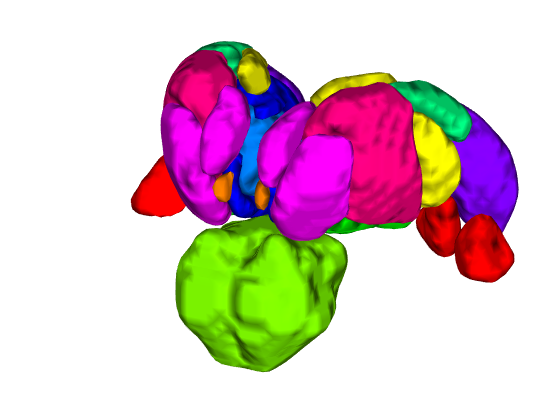
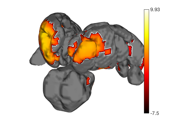
Here's a simple example visualizing all of the parcels in an atlas as 3-D blobs:
t = ttest(pain, .01, 'unc');

atlas_obj = load_atlas('thalamus');

create_figure('isosurface');
surface_handles = isosurface(atlas_obj);

% Now we'll set some lighting and figure properties
axis image vis3d off
material dull
view(210, 20);
lightRestoreSingle

drawnow, snapnow

% You can render blobs on these surfaces too.

render_on_surface(t, surface_handles, 'colormap', 'hot');
drawnow, snapnow
One-sample t-test
Calculating t-statistics and p-values

Image   1
230 contig. clusters, sizes   1 to 23979
Positive effect: 17159 voxels, min p-value: 0.00000000
Negative effect: 29798 voxels, min p-value: 0.00000000
Warning: This atlas is deprecated. Please specify thalamus_[fsl6|fmriprep20]
instead.
Loading atlas: /home/bogdan/.matlab/canlab/Neuroimaging_Pattern_Masks/Atlases_and_parcellations/2018_Wager_combined_atlas/Thalamus_combined_atlas_object.mat

ans =

  Light with properties:

       Color: [1 1 1]
       Style: 'infinite'
    Position: [-0.6645 1.1509 0.4837]
     Visible: on

  Use GET to show all properties
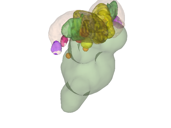
Let's load another atlas, and pull out all the "default mode" regions We'll use isosurface to visualize these
atlas_obj = load_atlas('canlab2018_2mm');
atlas_obj = select_atlas_subset(atlas_obj, {'Def'}, 'labels_2');

create_figure('isosurface');
surface_handles = isosurface(atlas_obj);

% let's add a cortical surface for context
% We'll make the back surface (right) opaque, and the front (left) transparent
han = addbrain('hires right');
set(han, 'FaceAlpha', 1);

han2 = addbrain('hires left');
set(han2, 'FaceAlpha', 0.1);

axis image vis3d off
material dull
view(-88, 31);
lightRestoreSingle

drawnow, snapnow
Loading atlas: CANlab_combined_atlas_object_2018_2mm.mat

ans =

  Light with properties:

       Color: [1 1 1]
       Style: 'infinite'
    Position: [-1.2115 -0.0423 0.7284]
     Visible: on

  Use GET to show all properties

Using isosurface to create a custom surface
You can build a cutaway surface or a series of them with the isosurface method, from any suitable image. The image used here is a mean anatomical image that renders nicely. As always, you can use Matlab's rendering to change the look of the surfaces
anat = fmri_data(which('keuken_2014_enhanced_for_underlay.img'), 'noverbose');

create_figure('cutaways'); axis off

surface_handles = isosurface(anat, 'thresh', 140, 'nosmooth', 'xlim', [-Inf 0], 'YLim', [-30 Inf], 'ZLim', [-Inf 40]);

axes(get(surface_handles(1),'Parent'))
view(-127, 33);
set(surface_handles, 'FaceAlpha', .85);

render_on_surface(t, surface_handles);

snapnow

Explore on your own
1. Try to create your own custom brain surface to visualize one of the 3 statistic image maps we've been working on. Can you make a plot that really shows the important results in a clear way?
2. Try exploring movie_tools to create a movie where you rotate, zoom, and change the transparency of your surfaces in some way. You can write movie files to disk for use in presentations, too.
3. Try rendering another atlas, or subset of an atlas, with isosurface() Maybe you can pull out and render all the "ventral attention" network regions.
Explore More: CANlab Toolboxes
Tutorials, overview, and help: https://canlab.github.io
Toolboxes and image repositories on github: https://github.com/canlab
| CANlab Core Tools | https://github.com/canlab/CanlabCore | CANlab Neuroimaging_Pattern_Masks repository | https://github.com/canlab/Neuroimaging_Pattern_Masks | CANlab_help_examples | https://github.com/canlab/CANlab_help_examples | M3 Multilevel mediation toolbox | https://github.com/canlab/MediationToolbox | M3 CANlab robust regression toolbox | https://github.com/canlab/RobustToolbox | M3 MKDA coordinate-based meta-analysis toolbox | https://github.com/canlab/Canlab_MKDA_MetaAnalysis |
Here are some other useful CANlab-associated resources:
| Paradigms_Public - CANlab experimental paradigms | https://github.com/canlab/Paradigms_Public | FMRI_simulations - brain movies, effect size/power | https://github.com/canlab/FMRI_simulations | CANlab_data_public - Published datasets | https://github.com/canlab/CANlab_data_public | M3 Neurosynth: Tal Yarkoni | https://github.com/neurosynth/neurosynth | M3 DCC - Martin Lindquist's dynamic correlation tbx | https://github.com/canlab/Lindquist_Dynamic_Correlation | M3 CanlabScripts - in-lab Matlab/python/bash | https://github.com/canlab/CanlabScripts |
Object-oriented, interactive approach The core basis for interacting with CANlab tools is through object-oriented framework. A simple set of neuroimaging data-specific objects (or classes) allows you to perform interactive analysis using simple commands (called methods) that operate on objects.
Map of core object classes:
