Regression Walkthrough
Contents
- Part 1: Load sample data
- Part 2: Examine the setup and coverage
- Part 3: Examine the brain data
- Part 4: Examine the behavioral/task predictor(s)
- Part 5: Make data prep and analysis decisions
- Part 6: Run the regression analysis and get results
- Write the thesholded t-image to disk
- Part 7. Explore: Display regions at a lower threshold, alongside meta-analysis regions
- Part 8: Compare to a standard analysis with no scaling or variable transformation
- Make plots comparing the analysis with our choices and a naive analysis directly
- Part 9: Localize results using a brain atlas
- Part 10: Extract and plot data from regions of interest
- Extract and plot from (biased) regions of interest based on results
- Extract and plot data from unbiased regions of interest
- Part 11: (bonus) Multivariate prediction from unbiased ROI averages
This walkthrough works through multiple aspects of a basic 2nd-level (group) analysis. We are interested in activity related to emotion regulation for a contrast comparing reappraisal of negative images vs. looking at negative images without reappraisal, i.e., a [Reappraise Negative - Look Negative] contrast. This walkthrough will regress brain contrast values in each voxel (y) onto individual differences in "Reappraisal Success", defined as the drop in negative emotion ratings for the [Reappraise Negative - Look Negative] contrast.
We are interested in both the brain correlates of individual differences and the group-average [Reappraise Negative - Look Negative] effect in the brain, which is the intercept in our regression model.
This walkthrough includes multiple considerations you'll need when doing a practical data analysis. This goes far beyond just running a model! It's also important to understand the data and results. Understanding the data allows you to make informed a priori choices about the analysis and avoid "P-Hacking". Understanding the results helps ensure they are valid, and helps you interpret them.
A) Understanding the data
- Loading the dataset into an fmri_data object
- Examining the brain data and checking
outliers
global signal
which voxels are analyzed (coverage)
homogeneity across subjects (images)
- Examining the behavioral (individual differences) data and leverages
- Use the info gained to make data preparation and analysis decisions
Masking
Transformation of the y variable
Rescaling/normalizing image data
Robust vs. OLS estimation
B) Fitting the model
- Running the regression and writing results images to disk
C) Understanding the results
- Explore variations in statistical threshold
- Compare with other studies by comparing with a meta-analysis mask
- Explore the impact of variations in data scaling/transformation
- Localizing results, labeling regions, and making tables using a brain atlas
- Extract and plot data from regions of interest
- Explore the impact of plotting data in biased vs. unbiased regions of interest
D) Multivariate prediction (overlaps with later walkthroughs) # Extra: Multivariate prediction within a set of unbiased ROIs
Part 1: Load sample data
Load a sample dataset, including a standard brain mask And a meta-analysis mask that provides a priori regions of interest. ---------------------------------------------------------------
% Load sample data using load_image_set(), which produces an fmri_data
% object. Data loading exceeds the scope of this tutorial, but a more
% indepth demosntration may be provided by canlab_help_2_load_a_sample_dataset.m

% These are [Reappraise - Look Neg] contrast images, one image per person

[image_obj, networknames, imagenames] = load_image_set('emotionreg');

% Summarize and print a table with characteristics of the data:
desc = descriptives(image_obj);

% Load behavioral data
% This is "Reappraisal success", one score per person, in our example
% If you do not have the file on your path, you will get an error.

beh = importdata('Wager_2008_emotionreg_behavioral_data.txt')
success = beh.data(:, 2);           % Reappraisal success

% Load a mask that we would like to apply to analysis/results

mask = which('gray_matter_mask.img')

maskdat = fmri_data(mask, 'noverbose');

% Map of emotion-regulation related regions from neurosynth.org
metaimg = which('emotion regulation_pAgF_z_FDR_0.01_8_14_2015.nii')

metamask = fmri_data(metaimg, 'noverbose');
Loaded images:
/Users/torwager/Documents/GitHub/CanlabCore/CanlabCore/Sample_datasets/Wager_et_al_2008_Neuron_EmotionReg/Wager_2008_emo_reg_vs_look_neg_contrast_images.nii
/Users/torwager/Documents/GitHub/CanlabCore/CanlabCore/Sample_datasets/Wager_et_al_2008_Neuron_EmotionReg/Wager_2008_emo_reg_vs_look_neg_contrast_images.nii
/Users/torwager/Documents/GitHub/CanlabCore/CanlabCore/Sample_datasets/Wager_et_al_2008_Neuron_EmotionReg/Wager_2008_emo_reg_vs_look_neg_contrast_images.nii
/Users/torwager/Documents/GitHub/CanlabCore/CanlabCore/Sample_datasets/Wager_et_al_2008_Neuron_EmotionReg/Wager_2008_emo_reg_vs_look_neg_contrast_images.nii
/Users/torwager/Documents/GitHub/CanlabCore/CanlabCore/Sample_datasets/Wager_et_al_2008_Neuron_EmotionReg/Wager_2008_emo_reg_vs_look_neg_contrast_images.nii
/Users/torwager/Documents/GitHub/CanlabCore/CanlabCore/Sample_datasets/Wager_et_al_2008_Neuron_EmotionReg/Wager_2008_emo_reg_vs_look_neg_contrast_images.nii
/Users/torwager/Documents/GitHub/CanlabCore/CanlabCore/Sample_datasets/Wager_et_al_2008_Neuron_EmotionReg/Wager_2008_emo_reg_vs_look_neg_contrast_images.nii
/Users/torwager/Documents/GitHub/CanlabCore/CanlabCore/Sample_datasets/Wager_et_al_2008_Neuron_EmotionReg/Wager_2008_emo_reg_vs_look_neg_contrast_images.nii
/Users/torwager/Documents/GitHub/CanlabCore/CanlabCore/Sample_datasets/Wager_et_al_2008_Neuron_EmotionReg/Wager_2008_emo_reg_vs_look_neg_contrast_images.nii
/Users/torwager/Documents/GitHub/CanlabCore/CanlabCore/Sample_datasets/Wager_et_al_2008_Neuron_EmotionReg/Wager_2008_emo_reg_vs_look_neg_contrast_images.nii
/Users/torwager/Documents/GitHub/CanlabCore/CanlabCore/Sample_datasets/Wager_et_al_2008_Neuron_EmotionReg/Wager_2008_emo_reg_vs_look_neg_contrast_images.nii
/Users/torwager/Documents/GitHub/CanlabCore/CanlabCore/Sample_datasets/Wager_et_al_2008_Neuron_EmotionReg/Wager_2008_emo_reg_vs_look_neg_contrast_images.nii
/Users/torwager/Documents/GitHub/CanlabCore/CanlabCore/Sample_datasets/Wager_et_al_2008_Neuron_EmotionReg/Wager_2008_emo_reg_vs_look_neg_contrast_images.nii
/Users/torwager/Documents/GitHub/CanlabCore/CanlabCore/Sample_datasets/Wager_et_al_2008_Neuron_EmotionReg/Wager_2008_emo_reg_vs_look_neg_contrast_images.nii
/Users/torwager/Documents/GitHub/CanlabCore/CanlabCore/Sample_datasets/Wager_et_al_2008_Neuron_EmotionReg/Wager_2008_emo_reg_vs_look_neg_contrast_images.nii
/Users/torwager/Documents/GitHub/CanlabCore/CanlabCore/Sample_datasets/Wager_et_al_2008_Neuron_EmotionReg/Wager_2008_emo_reg_vs_look_neg_contrast_images.nii
/Users/torwager/Documents/GitHub/CanlabCore/CanlabCore/Sample_datasets/Wager_et_al_2008_Neuron_EmotionReg/Wager_2008_emo_reg_vs_look_neg_contrast_images.nii
/Users/torwager/Documents/GitHub/CanlabCore/CanlabCore/Sample_datasets/Wager_et_al_2008_Neuron_EmotionReg/Wager_2008_emo_reg_vs_look_neg_contrast_images.nii
/Users/torwager/Documents/GitHub/CanlabCore/CanlabCore/Sample_datasets/Wager_et_al_2008_Neuron_EmotionReg/Wager_2008_emo_reg_vs_look_neg_contrast_images.nii
/Users/torwager/Documents/GitHub/CanlabCore/CanlabCore/Sample_datasets/Wager_et_al_2008_Neuron_EmotionReg/Wager_2008_emo_reg_vs_look_neg_contrast_images.nii
/Users/torwager/Documents/GitHub/CanlabCore/CanlabCore/Sample_datasets/Wager_et_al_2008_Neuron_EmotionReg/Wager_2008_emo_reg_vs_look_neg_contrast_images.nii
/Users/torwager/Documents/GitHub/CanlabCore/CanlabCore/Sample_datasets/Wager_et_al_2008_Neuron_EmotionReg/Wager_2008_emo_reg_vs_look_neg_contrast_images.nii
/Users/torwager/Documents/GitHub/CanlabCore/CanlabCore/Sample_datasets/Wager_et_al_2008_Neuron_EmotionReg/Wager_2008_emo_reg_vs_look_neg_contrast_images.nii
/Users/torwager/Documents/GitHub/CanlabCore/CanlabCore/Sample_datasets/Wager_et_al_2008_Neuron_EmotionReg/Wager_2008_emo_reg_vs_look_neg_contrast_images.nii
/Users/torwager/Documents/GitHub/CanlabCore/CanlabCore/Sample_datasets/Wager_et_al_2008_Neuron_EmotionReg/Wager_2008_emo_reg_vs_look_neg_contrast_images.nii
/Users/torwager/Documents/GitHub/CanlabCore/CanlabCore/Sample_datasets/Wager_et_al_2008_Neuron_EmotionReg/Wager_2008_emo_reg_vs_look_neg_contrast_images.nii
/Users/torwager/Documents/GitHub/CanlabCore/CanlabCore/Sample_datasets/Wager_et_al_2008_Neuron_EmotionReg/Wager_2008_emo_reg_vs_look_neg_contrast_images.nii
/Users/torwager/Documents/GitHub/CanlabCore/CanlabCore/Sample_datasets/Wager_et_al_2008_Neuron_EmotionReg/Wager_2008_emo_reg_vs_look_neg_contrast_images.nii
/Users/torwager/Documents/GitHub/CanlabCore/CanlabCore/Sample_datasets/Wager_et_al_2008_Neuron_EmotionReg/Wager_2008_emo_reg_vs_look_neg_contrast_images.nii
/Users/torwager/Documents/GitHub/CanlabCore/CanlabCore/Sample_datasets/Wager_et_al_2008_Neuron_EmotionReg/Wager_2008_emo_reg_vs_look_neg_contrast_images.nii

Source: Info about image source here


Summary of dataset
______________________________________________________
Images:  30	Nonempty:  30	Complete:  30
Voxels: 49792	Nonempty: 49792	Complete: 49245
Unique data values: 1481293

Min: -25.515	Max: 15.935	Mean: 0.159	Std: 1.382

    Percentiles     Values
    ___________    ________

        0.1         -8.3774
        0.5          -5.083
          1         -3.9722
          5         -1.8634
         25        -0.39993
         50         0.08903
         75         0.75436
         95          2.2821
         99          4.0183
       99.5          4.8676
       99.9           6.987


beh =

  struct with fields:

          data: [30×2 double]
      textdata: {'X_RVLPFC'  'Y_Reappraisal_Success'}
    colheaders: {'X_RVLPFC'  'Y_Reappraisal_Success'}


mask =

    '/Users/torwager/Documents/GitHub/CanlabCore/CanlabCore/canlab_canonical_brains/Canonical_brains_surfaces/gray_matter_mask.img'


metaimg =

    '/Users/torwager/Documents/GitHub/MediationToolbox/Mediation_walkthrough/emotion regulation_pAgF_z_FDR_0.01_8_14_2015.nii'
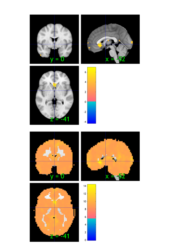
Part 2: Examine the setup and coverage
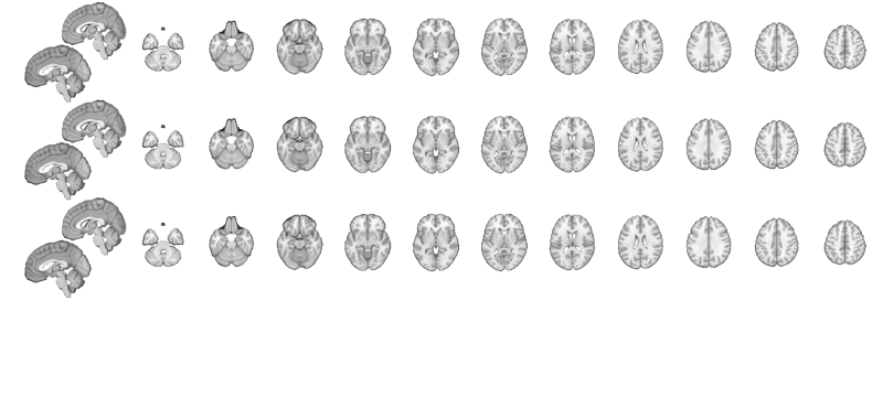
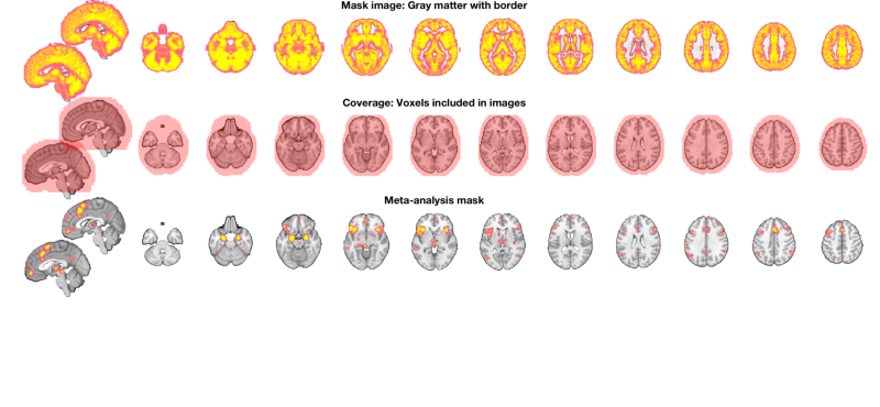
% Visualize the mask
% ---------------------------------------------------------------
% BLOCK 2: Check mask

% This is an underlay brain with three separate montages so we can compare images:

o2 = canlab_results_fmridisplay([], 'noverbose', 'multirow', 3);
drawnow, snapnow;

% This is a basic gray-matter mask we will use for analysis:
% It can help reduce multiple comparisons relative to whole-image analysis
% but we should still look at what's happening in ventricles and
% out-of-brain space to check for artifacts.

o2 = addblobs(o2, region(maskdat), 'wh_montages', 1:2);

% Add a title to montage 2, the axial slice montage:
[o2, title_han] = title_montage(o2, 2, 'Mask image: Gray matter with border');
set(title_han, 'FontSize', 18)

% Visualize summary of brain coverage
% ---------------------------------------------------------------
% Check that we have valid data in most voxels for most subjects
% Always look at which voxels you are analyzing. The answer may surprise
% you!  Some software programs mask out voxels in individual analyses,
% which may then be excluded in the group analysis.

% Show summary of coverage - how many images have non-zero, non-NaN values in each voxel

o2 = montage(region(desc.coverage_obj), o2, 'trans', 'transvalue', .3, 'wh_montages', 3:4);

[o2, title_han] = title_montage(o2, 4, 'Coverage: Voxels included in images');
set(title_han, 'FontSize', 18)

% Visualize meta-analysis mask
% ---------------------------------------------------------------
o2 = montage(region(metamask), o2, 'colormap', 'wh_montages', 5:6);

[o2, title_han] = title_montage(o2, 6, 'Meta-analysis mask');
set(title_han, 'FontSize', 18)

% There are many other alternatives to the montage - e.g.,:
% orthviews(desc.coverage_obj, 'continuous');
Grouping contiguous voxels:  46 regions
sagittal montage: 8208 voxels displayed, 203131 not displayed on these slices
axial montage: 42172 voxels displayed, 169167 not displayed on these slices
Grouping contiguous voxels:   1 regions
Grouping contiguous voxels: 151 regions
sagittal montage: 451 voxels displayed, 5590 not displayed on these slices
axial montage: 1579 voxels displayed, 4462 not displayed on these slices
Part 3: Examine the brain data
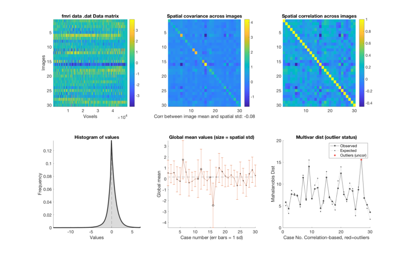
This is a really important step to understand what your images look like! Good data tend to produce good results.
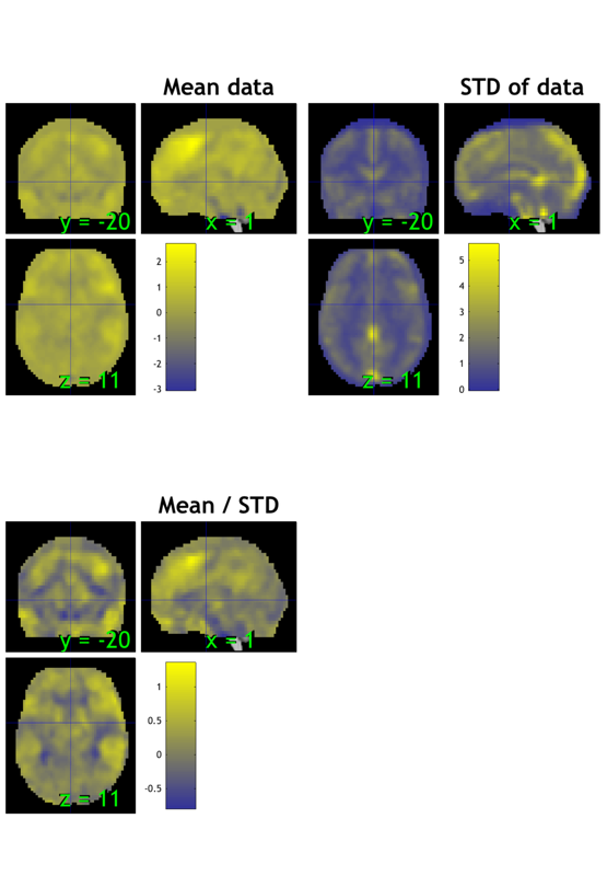
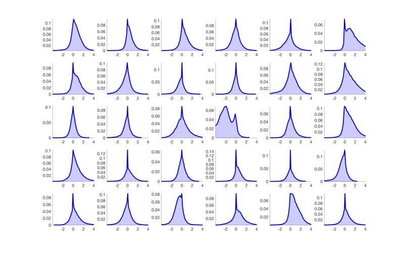
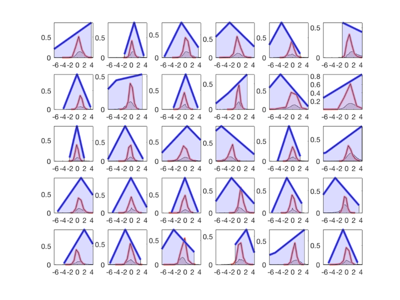
% The method plot() for an fmri_data object shows a number of plots that
% are helpful in diagnosing some problems.

plot(image_obj);

% Check histograms of individual subjects for global shifts in contrast values

% The 'histogram' object method will allow you to examine a series of
% images in one panel each.  See help fmri_data.histogram for more options,
% including breakdown by tissue type.

hist_han = histogram(image_obj, 'byimage', 'color', 'b');

% This shows us that some of the images do not have the same mean as the
% others. This is fairly common, as individual subjects can often have
% global artifacts (e.g., task-correlated head motion or outliers) that
% influence the whole contrast image, even when baseline conditions are
% supposed to be "subtracted out".
%
% It suggests that we may want to do an outlier analysis and/or standardize
% the scale of the images. We'll return to this below.

% If we want to visualize this separated by tissue class, try this:

create_figure('histogram by tissue type')
hist_han = histogram(image_obj, 'byimage', 'by_tissue_type');

% Our previous peek at the data suggested that subjects 6 and 16 have
% whole-brain shifts towards acftivation and deactivation, respectively.

% This plot shows us that there is a substantial shift in gray matter values
% across the brain for some individuals.
% Also, the means across gray and white matter are correlated.  So are the standard deviations.
% We might consider a rescaling or nonparametric procedure (e.g., ranking)
% to standardize the images.

% Some options are here:
help image_obj.rescale
Calculating mahalanobis distances to identify extreme-valued images
Retained 8 components for mahalanobis distance
Expected 50% of points within 50% normal ellipsoid, found 46.67%
Expected 1.50 outside 95% ellipsoid, found 1
Potential outliers based on mahalanobis distance:
Bonferroni corrected: 0 images Cases
Uncorrected: 1 images Cases 27
Outliers:
Outliers after p-value correction:
Image numbers:
Image numbers, uncorrected: 27
Warning: Ignoring extra legend entries.
Grouping contiguous voxels: 1 regions
Grouping contiguous voxels: 1 regions
Grouping contiguous voxels: 1 regions
ans =
Figure (histogram by tissue type) with properties:
Number: 5
Name: 'histogram by tissue type'
Color: [1 1 1]
Position: [680 558 560 420]
Units: 'pixels'
Use GET to show all properties
Extracting from gray_matter_mask_sparse.img.
Extracting from canonical_white_matter.img.
Extracting from canonical_ventricles.img.
------------------------------------------------------------
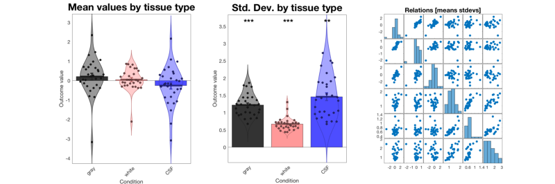
Plotting mean values by tissue type
Gray = gray, red = white, blue = CSF
Col 1: gray Col 2: white Col 3: CSF
---------------------------------------------
Tests of column means against zero
---------------------------------------------
Name Mean_Value Std_Error T P Cohens_d
_______ __________ _________ _______ _______ ________
'gray' 0.21392 0.17152 1.2472 0.2223 0.22771
'white' 0.056209 0.10298 0.54584 0.58935 0.099657
'CSF' -0.24914 0.18332 -1.3591 0.1846 -0.24813
------------------------------------------------------------
Plotting spatial standard deviations across voxels by tissue type
Gray = gray, red = white, blue = CSF
Col 1: gray Col 2: white Col 3: CSF
---------------------------------------------
Tests of column means against zero
---------------------------------------------
Name Mean_Value Std_Error T P Cohens_d
_______ __________ _________ ______ __________ ________
'gray' 1.2234 0.057213 21.383 2.2204e-15 3.904
'white' 0.67452 0.033531 20.116 2.2204e-15 3.6727
'CSF' 1.462 0.10912 13.399 5.9478e-14 2.4462
--- help for fmri_data/rescale ---
Rescales data in an fmri_data object
Data is observations x images, so operating on the columns operates on
images, and operating on the rows operates on voxels (or variables more
generally) across images.
:Usage:
::
fmridat = rescale(fmridat, meth)
:Inputs:
**Methods:**
Rescaling of voxels
- centervoxels subtract voxel means
- zscorevoxels subtract voxel means, divide by voxel std. dev
- rankvoxels replace values in each voxel with rank across images
Rescaling of images
- centerimages subtract image means
- zscoreimages subtract image means, divide by image std. dev
- l2norm_images divide each image by its l2 norm, multiply by sqrt(n valid voxels)
- divide_by_csf_l2norm divide each image by CSF l2 norm. requires MNI space images for ok results!
- rankimages rank voxels within image;
- csf_mean_var Subtract mean CSF signal from image and divide by CSF variance. (Useful for PE
maps where CSF mean and var should be 0).
Other procedures
- windsorizevoxels Winsorize extreme values to 3 SD for each image (separately) using trimts
- percentchange Scale each voxel (column) to percent signal change with a mean of 100
based on smoothed mean values across space (cols), using iimg_smooth_3d
- tanh Rescale variables by hyperbolic tangent function
this will shrink the tails (and outliers) towards the mean,
making subsequent algorithms more robust to
outliers. Affects normality of distribution.
Appropriate for multi-session (time series) only:
- session_global_percent_change
- session_global_z
- session_multiplicative
See also fmri_data.preprocess
Part 4: Examine the behavioral/task predictor(s)
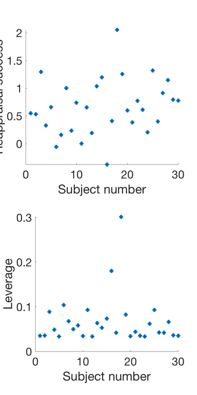
Examine predictor distribution and leverages Leverage is a measure of how much each point influences the regression line. The more extreme the predictor value, the higher the leverage. Outliers will have very high leverage. High-leverage behavioral observations can strongly influence, and sometimes invalidate, an analysis.
X = scale(success, 1); X(:, end+1) = 1;         % A simple design matrix, behavioral predictor + intercept
H = X * inv(X'* X) * X';                        % The "Hat Matrix", which produces fits. Diagonals are leverage

create_figure('levs', 2, 1);
plot(success, 'o', 'MarkerFaceColor', [0 .3 .7], 'LineWidth', 3);
set(gca, 'FontSize', 24);
xlabel('Subject number');
ylabel('Reappraisal success');

subplot(2, 1, 2);
plot(diag(H), 'o', 'MarkerFaceColor', [0 .3 .7], 'LineWidth', 3);
set(gca, 'FontSize', 24);
xlabel('Subject number');
ylabel('Leverage');

drawnow, snapnow

% The distribution suggests that there are some high-leverage values to
% watch out for. They will influence the results disproportionately at every voxel in the brain!
% Ranking predictors and/or robust regression are good
% mitigation/prevention procedures in many cases.
Part 5: Make data prep and analysis decisions
Before we've "peeked" at the results, let's make some sensible decisions about what to do with the analysis. We'll compare the results to the "standard analysis" if we hadn't examined the data at all at end.
% Choices:

% 1. Masking: Apply a gray-matter mask. This will limit the area subjected to multiple-comparisons
%    correction to a meaningful set.  I considered {gray matter, no mask}

image_obj = apply_mask(image_obj, maskdat);         % Mask - analyze gray-matter

% 2. Image scaling: I considered arbitrary rescaling of images, e.g., by
% the l2norm or z-scoring images. Z-scoring can cause artifactual
% de-activations when we are looking at group effects. L2-norming is
% sensible if there are bad scaling problems... but I'd rather minimize ad
% hoc procedures applied to the data. Ranking each voxel is also sensible, and
% if the predictor is ranked as well, this would implement Spearman's correlations.
% I considered {none, l2norm images, zscoreimages, rankvoxels}, and decided
% on ranking voxels.  For the group average (intercept), this is not  -- I'll use robust regression to help mitigate issues.

image_obj = rescale(image_obj, 'rankvoxels');     % rescale images within this mask (relative activation)

% 3. Predictor values: I considered dropping subject 16, which is a global
% outlier and also has high leverage, or windsorizing values to 3 sd.
% I also considered ranking predictor values, a very sensible choice.
% So I considered {do nothing, drop outlier, windsorize outliers, rank values}
% But robust regression (below) is partially redundant with this. I ultimately decided
% on ranking.

% This is done below:
% image_obj.X = scale(rankdata(image_obj.X), 1);

% 4. Regression method: I considered {standard OLS and robust IRLS
% regression}.  I chose robust regression because it helps mitigate the
% effects of outliers.  However, this is partly redundant with ranking, so
% it would have been sensible to choose ranking OR robust regression.
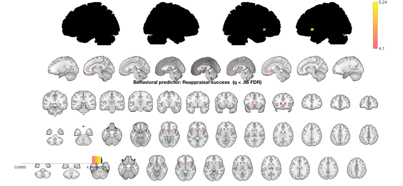
Part 6: Run the regression analysis and get results
The regress method takes predictors that are attached in the object's X attribute (X stands for design matrix) and regresses each voxel's activity (y) on the set of regressors. This is a group analysis, in this case correlating brain activity with reappraisal success at each voxel.
% .X must have the same number of observations, n, in an n x k matrix.
% n images is the number of COLUMNS in image_obj.dat

% mean-center success scores and attach them to image_obj in image_obj.X
image_obj.X = scale(success, 1);

image_obj.X = scale(rankdata(image_obj.X), 1);

% runs the regression at each voxel and returns statistic info and creates
% a visual image.  regress = multiple regression.
% % Track the time it takes (about 45 sec for robust regression on Tor's 2018 laptop)
tic

% out = regress(image_obj);             % this is what we'd do for standard OLS regression
out = regress(image_obj, 'robust');

toc

% out has statistic_image objects that have information about the betas
% (slopes) b, t-values and p-values (t), degrees of freedom (df), and sigma
% (error variance).  The critical one is out.t.
% out =
%
%         b: [1x1 statistic_image]
%         t: [1x1 statistic_image]
%        df: [1x1 fmri_data]
%     sigma: [1x1 fmri_data]

% This is a multiple regression, and there are two output t images, one for
% each regressor.  We've only entered one regressor, why two images?  The program always
% adds an intercept by default.  The intercept is always the last column of the design matrix

% Image   1  <--- brain contrast values correlated with "success"
% Positive effect:   0 voxels, min p-value: 0.00001192
% Negative effect:   0 voxels, min p-value: 0.00170529
% Image   2 FDR q < 0.050 threshold is 0.003193
%
% Image   2 <--- intercept, because we have mean-centered, this is the
% average group effect (when success = average success).  "Reapp - Look"
% contrast in the whole group.
% Positive effect: 3133 voxels, min p-value: 0.00000000
% Negative effect:  51 voxels, min p-value: 0.00024068

% Now let's try thresholding the image at q < .05 fdr-corrected.
t = threshold(out.t, .05, 'fdr');

% Select the predictor image we care about: (the 2nd/last image is the intercept)
t = select_one_image(t, 1);

% ...and display on a series of slices and surfaces
% There are many options for displaying results.
% montage and orthviews methods for statistic_image and region objects provide a good starting point.

o2 = montage(t, 'trans', 'full');
o2 = title_montage(o2, 2, 'Behavioral predictor: Reappraisal success  (q < .05 FDR)');
snapnow

% Or:
% orthviews(t)
Analysis:
----------------------------------
Design matrix warnings:
----------------------------------
No intercept detected, adding intercept to last column of design matrix

----------------------------------
Running regression: 34332 voxels. Design:  30 obs,   2 regressors, intercept is last

Predicting exogenous variable(s) in dat.X using brain data as predictors, mass univariate
Running in Robust Mode
Model run in 0 minutes and 44.32 seconds

Image   1
 40 contig. clusters, sizes   1 to  62
Positive effect: 156 voxels, min p-value: 0.00000016
Negative effect:   3 voxels, min p-value: 0.00022154

Image   2
 40 contig. clusters, sizes   1 to  62
Positive effect: 34332 voxels, min p-value: 0.00000000
Negative effect:   0 voxels, min p-value:
Elapsed time is 47.574783 seconds.
Image   1 FDR q < 0.050 threshold is 0.000048

Image   1
 11 contig. clusters, sizes   1 to  25
Positive effect:  35 voxels, min p-value: 0.00000016
Negative effect:   0 voxels, min p-value: 0.00022154
Image   2 FDR q < 0.050 threshold is 0.000000

Image   2
 11 contig. clusters, sizes   1 to  25
Positive effect: 34331 voxels, min p-value: 0.00000000
Negative effect:   0 voxels, min p-value:
Setting up fmridisplay objects
    48

Grouping contiguous voxels:  11 regions
Warning: Unknown input string option:full
sagittal montage:  27 voxels displayed,   8 not displayed on these slices
Warning: Unknown input string option:full
coronal montage:  15 voxels displayed,  20 not displayed on these slices
Warning: Unknown input string option:full
axial montage:  29 voxels displayed,   6 not displayed on these slices
Warning: Unknown input string option:full
axial montage:  16 voxels displayed,  19 not displayed on these slices
Write the thesholded t-image to disk
% % t.fullpath = fullfile(pwd, 'Reapp_Success_005_FDR05.nii');
% % write(t)
% %
% % disp(['Written to disk: ' t.fullpath])
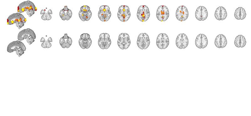
Part 7. Explore: Display regions at a lower threshold, alongside meta-analysis regions
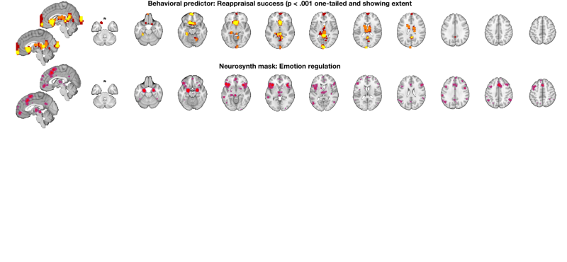
Display the results on slices another way: multi_threshold lets us see the blobs with significant voxels at the highest (most stringent) threshold, and voxels that are touching (contiguous) down to the lowest threshold, in different colors. This shows results at p < .001 one-tailed (p < .002 two-tailed), with 10 contiguous voxels. Contiguous blobs are more liberal thresholds, down to .02 two-tailed = .01 one tailed, are shown in different colors.
% Set up a display object with two separate brain montages:
o2 = canlab_results_fmridisplay([], 'multirow', 2);

% Use multi-threshold to threshold and display the t-map:
% Pass the fmridisplay object with montages (o2) in as an argument to use
% that for display.  Pass out the object with updated info.
% 'wh_montages', 1:2 tells it to plot only on the first two montages (one sagittal and one axial slice series)

o2 = multi_threshold(t, o2, 'thresh', [.002 .01 .02], 'sizethresh', [10 1 1], 'wh_montages', 1:2);
o2 = title_montage(o2, 2, 'Behavioral predictor: Reappraisal success (p < .001 one-tailed and showing extent');

% Get regions from map from neurosynth.org
% Defined above: metaimg = which('emotion regulation_pAgF_z_FDR_0.01_8_14_2015.nii')

r = region(metaimg);

% Add these to the bottom montages
o2 = addblobs(o2, r, 'maxcolor', [1 0 0], 'mincolor', [.7 .2 .5], 'wh_montages', 3:4);

o2 = title_montage(o2, 4, 'Neurosynth mask: Emotion regulation');

% Here, the regions predictive of success are largely different from those
% that respond to reappraisal demand in past literature.
Setting up fmridisplay objects

Multi-threshold
_____________________________________________
Retaining clusters contiguous with a significant cluster at p < 0.00200000 and k >=  10

Image   1 of   1
_____________________________________________
Threshold p < 0.00200000 and k >=  10	155 significant voxels defining blobs
Threshold p < 0.01000000 and k >=   1	452 significant voxels contiguous with a significant blob at a higher threshold
Threshold p < 0.02000000 and k >=   1	749 significant voxels contiguous with a significant blob at a higher threshold


Montage 1 of 1
_____________________________________
Warning: Unknown input string option:sizethresh
Warning: Unknown input string option:sizethresh
Warning: Unknown input string option:sizethresh
Warning: Unknown input string option:sizethresh
Warning: Unknown input string option:sizethresh
Warning: Unknown input string option:sizethresh
Grouping contiguous voxels: 151 regions
sagittal montage: 451 voxels displayed, 5590 not displayed on these slices
axial montage: 1579 voxels displayed, 4462 not displayed on these slices
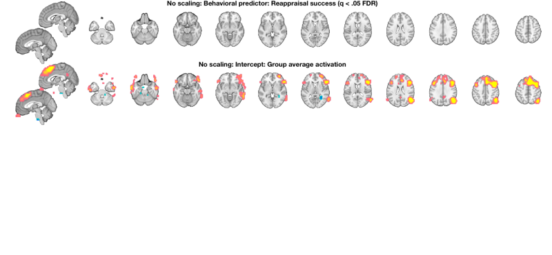
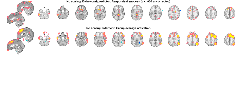
Part 8: Compare to a standard analysis with no scaling or variable transformation
% Start over and re-load the images:
[image_obj_untouched] = load_image_set('emotionreg', 'noverbose');

% attach success scores to image_obj in image_obj.X
% Just mean-center them so we can interpret the group result
image_obj_untouched.X = scale(success, 1);

% Do a standard OLS regression and view the results:
out = regress(image_obj_untouched, 'nodisplay');

% Treshold at q < .05 FDR and display
t_untouched = threshold(out.t, .05, 'fdr');

o2 = montage(t_untouched);
o2 = title_montage(o2, 2, 'No scaling: Behavioral predictor: Reappraisal success (q < .05 FDR)');
o2 = title_montage(o2, 4, 'No scaling: Intercept: Group average activation');

% Since we have no results for the predictor, re-threshold at p < .005
% uncorrected and display so we can see what's there:

t_untouched = threshold(t_untouched, .005, 'unc');

o2 = montage(t_untouched);
o2 = title_montage(o2, 2, 'No scaling: Behavioral predictor: Reappraisal success (p < .005 uncorrected)');
o2 = title_montage(o2, 4, 'No scaling: Intercept: Group average activation');
snapnow

% select just the image for reappraisal success:
t_untouched = select_one_image(t_untouched, 1);
Analysis:
----------------------------------
Design matrix warnings:
----------------------------------
No intercept detected, adding intercept to last column of design matrix

----------------------------------
Running regression: 49792 voxels. Design:  30 obs,   2 regressors, intercept is last

Predicting exogenous variable(s) in dat.X using brain data as predictors, mass univariate
Running in OLS Mode
Model run in 0 minutes and 0.08 seconds

Image   1
 24 contig. clusters, sizes   1 to  51
Positive effect: 203 voxels, min p-value: 0.00001192
Negative effect:   0 voxels, min p-value: 0.00170529

Image   2
 24 contig. clusters, sizes   1 to  51
Positive effect: 1969 voxels, min p-value: 0.00000000
Negative effect:  11 voxels, min p-value: 0.00024068
Image   1 FDR q < 0.050 threshold is 0.000000

Image   1
  0 contig. clusters, sizes  to
Positive effect:   0 voxels, min p-value: 0.00001192
Negative effect:   0 voxels, min p-value: 0.00170529
Image   2 FDR q < 0.050 threshold is 0.003193

Image   2
  0 contig. clusters, sizes  to
Positive effect: 3133 voxels, min p-value: 0.00000000
Negative effect:  51 voxels, min p-value: 0.00024068
Setting up fmridisplay objects
Grouping contiguous voxels:   0 regions
Grouping contiguous voxels:  28 regions
sagittal montage: 162 voxels displayed, 3022 not displayed on these slices
axial montage: 1617 voxels displayed, 1567 not displayed on these slices

Image   1
 67 contig. clusters, sizes   1 to 255
Positive effect: 1159 voxels, min p-value: 0.00001192
Negative effect:  10 voxels, min p-value: 0.00170529

Image   2
 67 contig. clusters, sizes   1 to 255
Positive effect: 3673 voxels, min p-value: 0.00000000
Negative effect:  75 voxels, min p-value: 0.00024068
Setting up fmridisplay objects
Grouping contiguous voxels:  67 regions
sagittal montage: 119 voxels displayed, 1050 not displayed on these slices
axial montage: 439 voxels displayed, 730 not displayed on these slices
Grouping contiguous voxels:  33 regions
sagittal montage: 191 voxels displayed, 3557 not displayed on these slices
axial montage: 1921 voxels displayed, 1827 not displayed on these slices
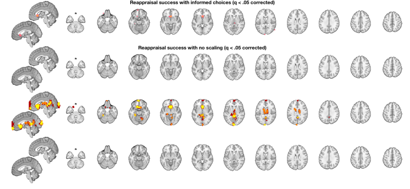
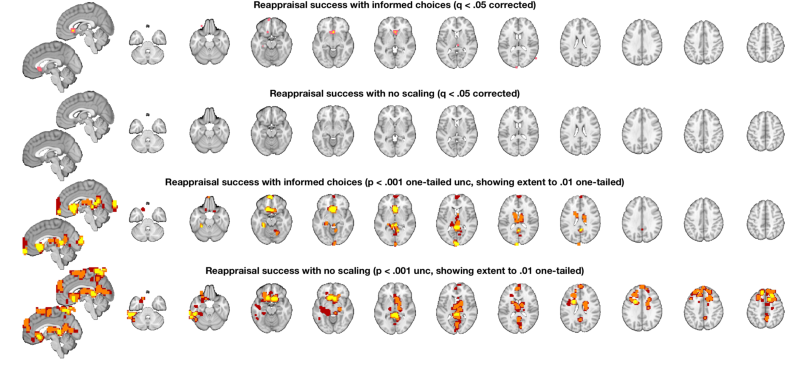
Make plots comparing the analysis with our choices and a naive analysis directly
o2 = canlab_results_fmridisplay([], 'multirow', 4);

t = threshold(t, .05, 'fdr');
o2 = montage(region(t), o2, 'wh_montages', 1:2, 'colormap');
o2 = title_montage(o2, 2, 'Reappraisal success with informed choices (q < .05 corrected)');

t_untouched = threshold(t_untouched, .05, 'fdr');
o2 = montage(region(t_untouched), o2, 'wh_montages', 3:4, 'colormap');
o2 = title_montage(o2, 4, 'Reappraisal success with no scaling (q < .05 corrected)');

% Here we'll use "multi-threshold" to display blobs at lower thresholds
% contiguous with those at higher thresholds. We'll use uncorrected p <
% .005 so we can see results in both maps:

o2 = multi_threshold(t, o2, 'thresh', [.002 .01 .02], 'k', [10 1 1], 'wh_montages', 5:6);
o2 = title_montage(o2, 6, 'Reappraisal success with informed choices (p < .001 one-tailed unc, showing extent to .01 one-tailed)');

o2 = multi_threshold(t_untouched, o2, 'thresh', [.002 .01 .02], 'k', [10 1 1], 'wh_montages', 7:8);
o2 = title_montage(o2, 8, 'Reappraisal success with no scaling (p < .001 unc, showing extent to .01 one-tailed)');

% One-tailed results are the default in SPM and FSL - so this is what you'd
% get with 0.001 in SPM.
Setting up fmridisplay objects
Image   1 FDR q < 0.050 threshold is 0.000048

Image   1
 11 contig. clusters, sizes   1 to  25
Positive effect:  35 voxels, min p-value: 0.00000016
Negative effect:   0 voxels, min p-value: 0.00022154
Grouping contiguous voxels:  11 regions
sagittal montage:  10 voxels displayed,  25 not displayed on these slices
axial montage:  29 voxels displayed,   6 not displayed on these slices
Image   1 FDR q < 0.050 threshold is 0.000000

Image   1
  0 contig. clusters, sizes  to
Positive effect:   0 voxels, min p-value: 0.00001192
Negative effect:   0 voxels, min p-value: 0.00170529
Grouping contiguous voxels:   0 regions

Multi-threshold
_____________________________________________
Retaining clusters contiguous with a significant cluster at p < 0.00200000 and k >=  10

Image   1 of   1
_____________________________________________
Threshold p < 0.00200000 and k >=  10	155 significant voxels defining blobs
Threshold p < 0.01000000 and k >=   1	452 significant voxels contiguous with a significant blob at a higher threshold
Threshold p < 0.02000000 and k >=   1	749 significant voxels contiguous with a significant blob at a higher threshold


Montage 1 of 1
_____________________________________
Multi-threshold
_____________________________________________
Retaining clusters contiguous with a significant cluster at p < 0.00200000 and k >=  10

Image   1 of   1
_____________________________________________
Threshold p < 0.00200000 and k >=  10	316 significant voxels defining blobs
Threshold p < 0.01000000 and k >=   1	1661 significant voxels contiguous with a significant blob at a higher threshold
Threshold p < 0.02000000 and k >=   1	3313 significant voxels contiguous with a significant blob at a higher threshold


Montage 1 of 1
_____________________________________

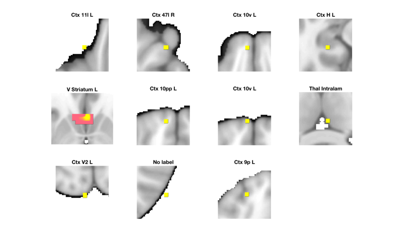
Part 9: Localize results using a brain atlas
The table() command is a simple way to label regions In addition, we can visualize each region in table to check the accuracy of the labels and the extent of the region.
% Select the Success regressor map
r = region(t);

% Autolabel regions and print a table
r = table(r);

% Make a montage showing each significant region
montage(r, 'colormap', 'regioncenters');
Grouping contiguous voxels:  11 regions

____________________________________________________________________________________________________________________________________________
Positive Effects
        Region         Volume            XYZ             maxZ      modal_label_descriptions      Perc_covered_by_label    Atlas_regions_covered    region_index
    _______________    ______    ___________________    ______    ___________________________    _____________________    _____________________    ____________

    'V_Striatum_L'      4448      -3      21      -5    5.2415    'Basal_ganglia'                         30                        1                    5
    'Ctx_47l_R'          480      38      34     -18    4.6608    'Cortex_Default_ModeB'                  33                        0                    2
    'Ctx_9p_L'           384     -24      45      36    5.0299    'Cortex_Default_ModeB'                  44                        0                   11
    'Ctx_H_L'            480     -31     -28     -14    4.7263    'Cortex_Default_ModeC'                  43                        0                    4
    'Ctx_10v_L'          352      -7      58     -18    4.5662    'Cortex_Limbic'                         89                        0                    3
    'Ctx_10pp_L'         344     -10      62     -14    4.5182    'Cortex_Limbic'                         91                        0                    6
    'Ctx_10v_L'          480      -7      69     -14     4.422    'Cortex_Limbic'                         40                        0                    7
    'Ctx_11l_L'          512     -28      41     -23    4.4234    'Cortex_Ventral_AttentionB'              8                        0                    1
    'Ctx_V2_L'           384      -7    -100      18    4.3753    'Cortex_Visual_Peripheral'              42                        0                    9
    'Thal_Intralam'      480       3     -24       9    4.5426    'Diencephalon'                          30                        1                    8
    'No label'           288      58     -69      18    4.5437    'No description'                         0                        0                   10


Negative Effects
No regions to display

____________________________________________________________________________________________________________________________________________
Regions labeled by reference atlas CANlab_2018_combined

Volume: Volume of contiguous region in cubic mm.
MaxZ: Signed max over Z-score for each voxel.
Atlas_regions_covered: Number of reference atlas regions covered at least 25% by the region. This relates to whether the region covers
multiple reference atlas regions
Region: Best reference atlas label, defined as reference region with highest number of in-region voxels. Regions covering >25% of >5
regions labeled as "Multiple regions"
Perc_covered_by_label: Percentage of the region covered by the label.
Ref_region_perc: Percentage of the label region within the target region.
modal_atlas_index: Index number of label region in reference atlas
all_regions_covered: All regions covered >5% in descending order of importance

For example, if a region is labeled 'TE1a' and Perc_covered_by_label = 8, Ref_region_perc = 38, and Atlas_regions_covered = 17, this means
that 8% of the region's voxels are labeled TE1a, which is the highest percentage among reference label regions. 38% of the region TE1a is
covered by the region. However, the region covers at least 25% of 17 distinct labeled reference regions.

References for atlases:

Beliveau, Vincent, Claus Svarer, Vibe G. Frokjaer, Gitte M. Knudsen, Douglas N. Greve, and Patrick M. Fisher. 2015. “Functional
Connectivity of the Dorsal and Median Raphe Nuclei at Rest.” NeuroImage 116 (August): 187–95.
Bär, Karl-Jürgen, Feliberto de la Cruz, Andy Schumann, Stefanie Koehler, Heinrich Sauer, Hugo Critchley, and Gerd Wagner. 2016. ?Functional
Connectivity and Network Analysis of Midbrain and Brainstem Nuclei.? NeuroImage 134 (July):53?63.
Diedrichsen, Jörn, Joshua H. Balsters, Jonathan Flavell, Emma Cussans, and Narender Ramnani. 2009. A Probabilistic MR Atlas of the Human
Cerebellum. NeuroImage 46 (1): 39?46.
Fairhurst, Merle, Katja Wiech, Paul Dunckley, and Irene Tracey. 2007. ?Anticipatory Brainstem Activity Predicts Neural Processing of Pain
in Humans.? Pain 128 (1-2):101?10.
Fan 2016 Cerebral Cortex; doi:10.1093/cercor/bhw157
Glasser, Matthew F., Timothy S. Coalson, Emma C. Robinson, Carl D. Hacker, John Harwell, Essa Yacoub, Kamil Ugurbil, et al. 2016. A
Multi-Modal Parcellation of Human Cerebral Cortex. Nature 536 (7615): 171?78.
Keren, Noam I., Carl T. Lozar, Kelly C. Harris, Paul S. Morgan, and Mark A. Eckert. 2009. “In Vivo Mapping of the Human Locus Coeruleus.”
NeuroImage 47 (4): 1261–67.
Keuken, M. C., P-L Bazin, L. Crown, J. Hootsmans, A. Laufer, C. Müller-Axt, R. Sier, et al. 2014. “Quantifying Inter-Individual Anatomical
Variability in the Subcortex Using 7 T Structural MRI.” NeuroImage 94 (July): 40–46.
Krauth A, Blanc R, Poveda A, Jeanmonod D, Morel A, Székely G. (2010) A mean three-dimensional atlas of the human thalamus: generation from
multiple histological data. Neuroimage. 2010 Feb 1;49(3):2053-62. Jakab A, Blanc R, Berényi EL, Székely G. (2012) Generation of
Individualized Thalamus Target Maps by Using Statistical Shape Models and Thalamocortical Tractography. AJNR Am J Neuroradiol. 33:
2110-2116, doi: 10.3174/ajnr.A3140
Nash, Paul G., Vaughan G. Macefield, Iven J. Klineberg, Greg M. Murray, and Luke A. Henderson. 2009. ?Differential Activation of the Human
Trigeminal Nuclear Complex by Noxious and Non-Noxious Orofacial Stimulation.? Human Brain Mapping 30 (11):3772?82.
Pauli 2018 Bioarxiv: CIT168 from Human Connectome Project data
Pauli, Wolfgang M., Amanda N. Nili, and J. Michael Tyszka. 2018. ?A High-Resolution Probabilistic in Vivo Atlas of Human Subcortical Brain
Nuclei.? Scientific Data 5 (April): 180063.
Pauli, Wolfgang M., Randall C. O?Reilly, Tal Yarkoni, and Tor D. Wager. 2016. ?Regional Specialization within the Human Striatum for
Diverse Psychological Functions.? Proceedings of the National Academy of Sciences of the United States of America 113 (7): 1907?12.
Sclocco, Roberta, Florian Beissner, Gaelle Desbordes, Jonathan R. Polimeni, Lawrence L. Wald, Norman W. Kettner, Jieun Kim, et al. 2016.
?Neuroimaging Brainstem Circuitry Supporting Cardiovagal Response to Pain: A Combined Heart Rate Variability/ultrahigh-Field (7 T)
Functional Magnetic Resonance Imaging Study.? Philosophical Transactions. Series A, Mathematical, Physical, and Engineering Sciences 374
(2067). rsta.royalsocietypublishing.org. https://doi.org/10.1098/rsta.2015.0189.
Shen, X., F. Tokoglu, X. Papademetris, and R. T. Constable. 2013. “Groupwise Whole-Brain Parcellation from Resting-State fMRI Data for
Network Node Identification.” NeuroImage 82 (November): 403–15.
Zambreanu, L., R. G. Wise, J. C. W. Brooks, G. D. Iannetti, and I. Tracey. 2005. ?A Role for the Brainstem in Central Sensitisation in
Humans. Evidence from Functional Magnetic Resonance Imaging.? Pain 114 (3):397?407.

Note: Region object r(i).title contains full list of reference atlas regions covered by each cluster.
____________________________________________________________________________________________________________________________________________

Part 10: Extract and plot data from regions of interest
Here, we'll explore data extracted from two kinds of regions:
% 1 - biased regions based on the significant results. This is good for
% visualizing the distribution of the data in a region and checking
% assumptions, but examining the correlation in these regions is
% "circular", as the correlation was used to select voxels in the first
% place. The observed correlations in these regions will be upwardly
% biased as a result. In general, you cannot estimate the effect size
% (correlation or other metric) in a region or voxel after selecting it
% using criteria that are non-independent of the effect of interest.

% 2 - unbiased regions from the meta-analysis.  These are fair.
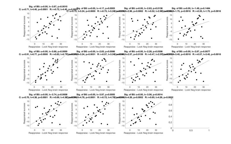
Extract and plot from (biased) regions of interest based on results
Here, we'll compare the implications of picking BIASED ROIs (which is often done in the literature) vs. picking UNBIASED ROIs.
First, let's visualize the correlation scatterplots in the areas we've discovered as related to Success
% Extract data from all regions
% r(i).dat has the averages for each subject across voxels for region i
r = extract_data(r, image_obj);

% Select only regions with 3+ voxels
% wh = cat(1, r.numVox) < 3;
% r(wh) = [];

% Set up the scatterplots
nrows = floor(sqrt(length(r)));
ncols = ceil(length(r) ./ nrows);
create_figure('scatterplot_region', nrows, ncols);

% Make a loop and plot each region
for i = 1:length(r)

    subplot(nrows, ncols, i);

    % Use this line for non-robust correlations:
    %plot_correlation_samefig(r(i).dat, datno16.X);

    % Use this line for robust correlations:
    plot_correlation_samefig(r(i).dat, image_obj.X, [], 'k', 0, 1);

    set(gca, 'FontSize', 12);
    xlabel('Reappraise - Look Neg brain response');
    ylabel('Reappraisal success');

    % input('Press a key to continue');

end
Warning: Iteration limit reached.
Warning: Iteration limit reached.
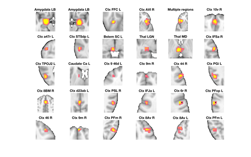
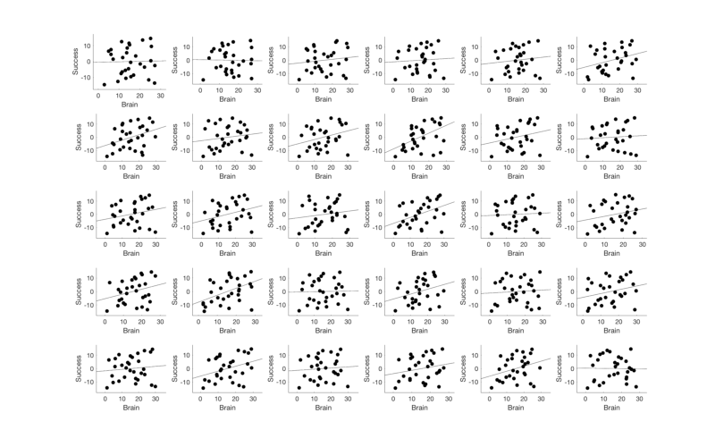
Extract and plot data from unbiased regions of interest
Let's visualize the correlation scatterplots in some meta-analysis derived ROIs
% Select the Neurosynth meta-analysis map
r = region(metaimg);

% Extract data from all regions
r = extract_data(r, image_obj);

% Select only regions with 20+ voxels
wh = cat(1, r.numVox) < 20;
r(wh) = [];

r = table(r);

% Make a montage showing each significant region
montage(r, 'colormap', 'regioncenters');

% Set up the scatterplots
nrows = floor(sqrt(length(r)));
ncols = ceil(length(r) ./ nrows);
create_figure('scatterplot_region', nrows, ncols);

% Make a loop and plot each region
for i = 1:length(r)

    subplot(nrows, ncols, i);

    % Use this line for non-robust correlations:
    %plot_correlation_samefig(r(i).dat, datno16.X);

    % Use this line for robust correlations:
    plot_correlation_samefig(r(i).dat, image_obj.X, [], 'k', 0, 1);

    set(gca, 'FontSize', 12);
    xlabel('Brain');
    ylabel('Success');
    title(' ');

end
Grouping contiguous voxels: 151 regions

____________________________________________________________________________________________________________________________________________
Positive Effects
          Region          Volume           XYZ            maxZ      modal_label_descriptions      Perc_covered_by_label    Atlas_regions_covered    region_index
    __________________    ______    _________________    ______    ___________________________    _____________________    _____________________    ____________

    'Amygdala_LB_'         4624     -22     -4    -16    7.0345    'Amygdala'                              24                        4                    1
    'Amygdala_LB_'         3664      24     -4    -16    7.0345    'Amygdala'                              36                        4                    2
    'Caudate_Ca_L'          208     -14      6     10    5.4136    'Basal_ganglia'                         73                        0                   14
    'Bstem_SC_L'            560      -4    -28     -4    7.0345    'Brainstem'                             44                        2                    9
    'Ctx_10v_R'            1192      -2     52     -8    7.0345    'Cortex_Default_ModeA'                  32                        0                    6
    'Ctx_9m_R'              160       0     62     18    4.7765    'Cortex_Default_ModeA'                  65                        0                   16
    'Ctx_d23ab_L'           408      -2    -52     28    6.0507    'Cortex_Default_ModeA'                  35                        0                   20
    'Ctx_9m_R'              296       4     56     32    6.0507    'Cortex_Default_ModeA'                  84                        0                   26
    'Ctx_STSdp_L'           632     -58    -36     -2    7.0345    'Cortex_Default_ModeB'                  43                        0                    8
    'Ctx_44_R'             1096      52     22     24    7.0345    'Cortex_Default_ModeB'                  39                        0                   17
    'Ctx_PGi_L'            1048     -52    -58     28    7.0345    'Cortex_Default_ModeB'                  50                        0                   18
    'Ctx_8Av_L'            1400     -40     12     46    7.0345    'Cortex_Default_ModeB'                  23                        0                   29
    'Ctx_FFC_L'             272     -42    -48    -18    6.6878    'Cortex_Dorsal_AttentionA'              76                        0                    3
    'Ctx_TPOJ2_L'           640     -52    -66      8    6.0507    'Cortex_Dorsal_AttentionA'              55                        0                   13
    'Ctx_PFop_L'            272     -62    -28     32    6.6878    'Cortex_Dorsal_AttentionB'              50                        0                   24
    'Ctx_IFJa_L'            528     -44     14     30    7.0345    'Cortex_Fronto_ParietalA'               52                        0                   22
    'Ctx_a47r_L'            360     -42     46    -10    7.0345    'Cortex_Fronto_ParietalB'               62                        0                    7
    'Ctx_8BM_R'            6872       0     18     44    7.0345    'Cortex_Fronto_ParietalB'               21                        4                   19
    'Ctx_PFm_R'             984      52    -50     42    7.0345    'Cortex_Fronto_ParietalB'               79                        0                   27
    'Ctx_8Av_R'             544      38     24     40    5.4136    'Cortex_Fronto_ParietalB'               38                        0                   28
    'Ctx_PFm_L'             344     -50    -52     42    6.0507    'Cortex_Fronto_ParietalB'               58                        0                   30
    'Ctx_PSL_R'             392      58    -44     28    6.0507    'Cortex_Temporal_Parietal'              63                        0                   21
    'Multiple regions'    10992     -42     22     -2    7.0345    'Cortex_Ventral_AttentionA'             14                        7                    5
    'Ctx_6r_R'              456      48      6     30    7.0345    'Cortex_Ventral_AttentionA'             46                        0                   23
    'Ctx_AVI_R'            4624      38     20     -4    7.0345    'Cortex_Ventral_AttentionB'             22                        2                    4
    'Ctx_IFSa_R'            528      52     30      8    6.0507    'Cortex_Ventral_AttentionB'             38                        0                   12
    'Ctx_9_46d_L'           168     -32     50     14    5.4136    'Cortex_Ventral_AttentionB'             62                        0                   15
    'Ctx_46_R'              232      34     40     30    5.4136    'Cortex_Ventral_AttentionB'             72                        0                   25
    'Thal_LGN'              280     -22    -26     -6    5.4136    'Diencephalon'                          37                        0                   10
    'Thal_MD'              1696      -2    -14      4    7.0345    'Diencephalon'                          57                        1                   11


Negative Effects
No regions to display

____________________________________________________________________________________________________________________________________________
Regions labeled by reference atlas CANlab_2018_combined

Volume: Volume of contiguous region in cubic mm.
MaxZ: Signed max over Input mask image values for each voxel.
Atlas_regions_covered: Number of reference atlas regions covered at least 25% by the region. This relates to whether the region covers
multiple reference atlas regions
Region: Best reference atlas label, defined as reference region with highest number of in-region voxels. Regions covering >25% of >5
regions labeled as "Multiple regions"
Perc_covered_by_label: Percentage of the region covered by the label.
Ref_region_perc: Percentage of the label region within the target region.
modal_atlas_index: Index number of label region in reference atlas
all_regions_covered: All regions covered >5% in descending order of importance

For example, if a region is labeled 'TE1a' and Perc_covered_by_label = 8, Ref_region_perc = 38, and Atlas_regions_covered = 17, this means
that 8% of the region's voxels are labeled TE1a, which is the highest percentage among reference label regions. 38% of the region TE1a is
covered by the region. However, the region covers at least 25% of 17 distinct labeled reference regions.

References for atlases:

Beliveau, Vincent, Claus Svarer, Vibe G. Frokjaer, Gitte M. Knudsen, Douglas N. Greve, and Patrick M. Fisher. 2015. “Functional
Connectivity of the Dorsal and Median Raphe Nuclei at Rest.” NeuroImage 116 (August): 187–95.
Bär, Karl-Jürgen, Feliberto de la Cruz, Andy Schumann, Stefanie Koehler, Heinrich Sauer, Hugo Critchley, and Gerd Wagner. 2016. ?Functional
Connectivity and Network Analysis of Midbrain and Brainstem Nuclei.? NeuroImage 134 (July):53?63.
Diedrichsen, Jörn, Joshua H. Balsters, Jonathan Flavell, Emma Cussans, and Narender Ramnani. 2009. A Probabilistic MR Atlas of the Human
Cerebellum. NeuroImage 46 (1): 39?46.
Fairhurst, Merle, Katja Wiech, Paul Dunckley, and Irene Tracey. 2007. ?Anticipatory Brainstem Activity Predicts Neural Processing of Pain
in Humans.? Pain 128 (1-2):101?10.
Fan 2016 Cerebral Cortex; doi:10.1093/cercor/bhw157
Glasser, Matthew F., Timothy S. Coalson, Emma C. Robinson, Carl D. Hacker, John Harwell, Essa Yacoub, Kamil Ugurbil, et al. 2016. A
Multi-Modal Parcellation of Human Cerebral Cortex. Nature 536 (7615): 171?78.
Keren, Noam I., Carl T. Lozar, Kelly C. Harris, Paul S. Morgan, and Mark A. Eckert. 2009. “In Vivo Mapping of the Human Locus Coeruleus.”
NeuroImage 47 (4): 1261–67.
Keuken, M. C., P-L Bazin, L. Crown, J. Hootsmans, A. Laufer, C. Müller-Axt, R. Sier, et al. 2014. “Quantifying Inter-Individual Anatomical
Variability in the Subcortex Using 7 T Structural MRI.” NeuroImage 94 (July): 40–46.
Krauth A, Blanc R, Poveda A, Jeanmonod D, Morel A, Székely G. (2010) A mean three-dimensional atlas of the human thalamus: generation from
multiple histological data. Neuroimage. 2010 Feb 1;49(3):2053-62. Jakab A, Blanc R, Berényi EL, Székely G. (2012) Generation of
Individualized Thalamus Target Maps by Using Statistical Shape Models and Thalamocortical Tractography. AJNR Am J Neuroradiol. 33:
2110-2116, doi: 10.3174/ajnr.A3140
Nash, Paul G., Vaughan G. Macefield, Iven J. Klineberg, Greg M. Murray, and Luke A. Henderson. 2009. ?Differential Activation of the Human
Trigeminal Nuclear Complex by Noxious and Non-Noxious Orofacial Stimulation.? Human Brain Mapping 30 (11):3772?82.
Pauli 2018 Bioarxiv: CIT168 from Human Connectome Project data
Pauli, Wolfgang M., Amanda N. Nili, and J. Michael Tyszka. 2018. ?A High-Resolution Probabilistic in Vivo Atlas of Human Subcortical Brain
Nuclei.? Scientific Data 5 (April): 180063.
Pauli, Wolfgang M., Randall C. O?Reilly, Tal Yarkoni, and Tor D. Wager. 2016. ?Regional Specialization within the Human Striatum for
Diverse Psychological Functions.? Proceedings of the National Academy of Sciences of the United States of America 113 (7): 1907?12.
Sclocco, Roberta, Florian Beissner, Gaelle Desbordes, Jonathan R. Polimeni, Lawrence L. Wald, Norman W. Kettner, Jieun Kim, et al. 2016.
?Neuroimaging Brainstem Circuitry Supporting Cardiovagal Response to Pain: A Combined Heart Rate Variability/ultrahigh-Field (7 T)
Functional Magnetic Resonance Imaging Study.? Philosophical Transactions. Series A, Mathematical, Physical, and Engineering Sciences 374
(2067). rsta.royalsocietypublishing.org. https://doi.org/10.1098/rsta.2015.0189.
Shen, X., F. Tokoglu, X. Papademetris, and R. T. Constable. 2013. “Groupwise Whole-Brain Parcellation from Resting-State fMRI Data for
Network Node Identification.” NeuroImage 82 (November): 403–15.
Zambreanu, L., R. G. Wise, J. C. W. Brooks, G. D. Iannetti, and I. Tracey. 2005. ?A Role for the Brainstem in Central Sensitisation in
Humans. Evidence from Functional Magnetic Resonance Imaging.? Pain 114 (3):397?407.

Note: Region object r(i).title contains full list of reference atlas regions covered by each cluster.
____________________________________________________________________________________________________________________________________________

Part 11: (bonus) Multivariate prediction from unbiased ROI averages
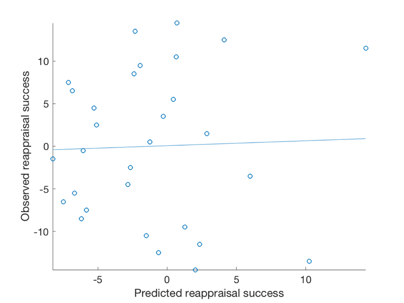
Predict reappraisal success using brain images with 5-fold cross-validation
% Since we are predicting outcome data from brain images, we have to attach
% data in the .Y field of the fmri_data object.
% .Y is the outcome to be explained, in this case success scores
image_obj.Y = image_obj.X;

% 5-fold cross validated prediction, stratified on outcome

[cverr, stats, optout] = predict(image_obj, 'algorithm_name', 'cv_lassopcrmatlab', 'nfolds', 5);

% Plot cross-validated predicted outcomes vs. actual

% Critical fields in stats output structure:
% stats.Y = actual outcomes
% stats.yfit = cross-val predicted outcomes
% pred_outcome_r: Correlation between .yfit and .Y
% weight_obj: Weight map used for prediction (across all subjects).

% Continuous outcomes:

create_figure('scatterplot');
plot(stats.yfit, stats.Y, 'o')
axis tight
refline
xlabel('Predicted reappraisal success');
ylabel('Observed reappraisal success');

% Though many areas show some significant effects, these are not strong
% enough to obtain a meaningful out-of-sample prediction of Success
Cross-validated prediction with algorithm cv_lassopcrmatlab,   5 folds
Regression mode (Gaussian)
Completed fit for all data in:   0 hours   0 min  0 secs
Regression mode (Gaussian) Fold 1/5 done in:   0 hours   0 min  0 sec
Regression mode (Gaussian) Fold 2/5 done in:   0 hours   0 min  0 sec
Regression mode (Gaussian) Fold 3/5 done in:   0 hours   0 min  0 sec
Regression mode (Gaussian) Fold 4/5 done in:   0 hours   0 min  0 sec
Regression mode (Gaussian) Fold 5/5 done in:   0 hours   0 min  0 sec

Total Elapsed Time =   0 hours   0 min  0 sec