Contents
- Load dataset with images and print descriptives
- Collect some variables we need
- Plot the ratings
- Prediction
- Run the Base model
- Plot the results
- Summarize within-person classification accuracy
- Visualize weight map
- Bootstrap weights: Get most reliable weights and p-values for voxels
- Try normalizing/scaling data
- Try selecting an a priori 'network of interest'
- re-run prediction and plot
- Other ideas
Dependencies:
% Matlab statistics toolbox
    % Matlab signal processing toolbox
    % Statistical Parametric Mapping (SPM) software https://www.fil.ion.ucl.ac.uk/spm/
    % For full functionality, the full suite of CANlab toolboxes is recommended. See here: Installing Tools
% About this dataset
% -------------------------------------------------------------------------
%
% This dataset includes 33 participants, with brain responses to six levels
% of heat (non-painful and painful).
%
% Aspects of this data appear in these papers:
% Wager, T.D., Atlas, L.T., Lindquist, M.A., Roy, M., Choong-Wan, W., Kross, E. (2013).
% An fMRI-Based Neurologic Signature of Physical Pain. The New England Journal of Medicine. 368:1388-1397
% (Study 2)
%
% Woo, C. -W., Roy, M., Buhle, J. T. & Wager, T. D. (2015). Distinct brain systems
% mediate the effects of nociceptive input and self-regulation on pain. PLOS Biology. 13(1):
% e1002036. doi:10.1371/journal.pbio.1002036
%
% Lindquist, Martin A., Anjali Krishnan, Marina López-Solà, Marieke Jepma, Choong-Wan Woo,
% Leonie Koban, Mathieu Roy, et al. 2015. ?Group-Regularized Individual Prediction:
% Theory and Application to Pain.? NeuroImage.
% http://www.sciencedirect.com/science/article/pii/S1053811915009982.
%
Load dataset with images and print descriptives
This dataset is shared on figshare.com, under this link: https://figshare.com/s/ca23e5974a310c44ca93
Here is a direct link to the dataset file with the fmri_data object: https://ndownloader.figshare.com/files/12708989
The key variable is image_obj This is an fmri_data object from the CANlab Core Tools repository for neuroimaging data analysis. See https://canlab.github.io/
image_obj.dat contains brain data for each image (average across trials) image_obj.Y contains pain ratings (one average rating per image)
image_obj.additional_info.subject_id contains integers coding for which Load the data file, downloading from figshare if needed
fmri_data_file = which('bmrk3_6levels_pain_dataset.mat');

if isempty(fmri_data_file)

    % attempt to download
    disp('Did not find data locally...downloading data file from figshare.com')

    fmri_data_file = websave('bmrk3_6levels_pain_dataset.mat', 'https://ndownloader.figshare.com/files/12708989');

end

load(fmri_data_file);

descriptives(image_obj);
Source: BMRK3 dataset from CANlab, PI Tor Wager
Data: .dat contains 6 images per participant, activation estimates during heat on L arm from level 1(44.3 degrees C) to level 6(49.3), in 1 degree increments.


____________________________________________________________________________________________________________________________________________
 Wager, T.D., Atlas, L.T., Lindquist, M.A., Roy, M., Choong-Wan, W., Kross, E. (2013). An fMRI-Based Neurologic Signature of Physical Pain.
The New England Journal of Medicine. 368:1388-1397 (Study 2)

 Woo, C. -W., Roy, M., Buhle, J. T. & Wager, T. D. (2015). Distinct brain systems mediate the effects of nociceptive input and
self-regulation on pain. PLOS Biology. 13(1): e1002036. doi:10.1371/journal.pbio.1002036

Lindquist, Martin A., Anjali Krishnan, Marina López-Solà, Marieke Jepma, Choong-Wan Woo, Leonie Koban, Mathieu Roy, et al. 2015.
“Group-Regularized Individual Prediction: Theory and Application to Pain.” NeuroImage.
http://www.sciencedirect.com/science/article/pii/S1053811915009982.

____________________________________________________________________________________________________________________________________________

Summary of dataset
______________________________________________________
Images: 198	Nonempty: 198	Complete: 198
Voxels: 223707	Nonempty: 223707	Complete: 223707
Unique data values: 35583281

Min: -11.529	Max: 7.862	Mean: -0.004	Std: 0.227

    Percentiles      Values
    ___________    __________

        0.1            -1.529
        0.5          -0.88055
          1          -0.67632
          5          -0.31891
         25         -0.087519
         50        0.00034864
         75          0.087461
         95           0.29757
         99           0.60449
       99.5           0.77676
       99.9            1.3177
Collect some variables we need
% subject_id is useful for cross-validation
%
% this used as a custom holdout set in fmri_data.predict() below will
% implement leave-one-subject-out cross-validation

subject_id = image_obj.additional_info.subject_id;

% ratings: reconstruct a subjects x temperatures matrix
% so we can plot it
%
% The command below does this only because we have exactly 6 conditions
% nested within 33 subjects and no missing data.

ratings = reshape(image_obj.Y, 6, 33)';

% temperatures are 44 - 49 (actually 44.3 - 49.3) in order for each person.

temperatures = image_obj.additional_info.temperatures;
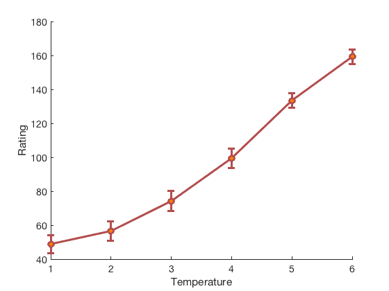
Plot the ratings
-------------------------------------------------------------------------
create_figure('ratings');
lineplot_columns(ratings, 'color', [.7 .3 .3], 'markerfacecolor', [1 .5 0]);
xlabel('Temperature');
ylabel('Rating');
Prediction
There are many options
% Base model: Linear, whole brain prediction
%
% Outcome distribution:
% Continuous: Regression (LASSO-PCR) Categorical/2 choice: SVM, logistic regression
%
% Model Options:
% - Feature selection (part of the brain)
% - Feature integration (new features)
%
% Testing options:
% - Input data (what level)
% - Cross-validation
% - What testing metric (classification accuracy? RMSE?) and at what level
% (single-trial, condition averages, one-map-per-subject)
%
% Inference options:
% - Component maps, voxel-wise maps
% - Thresholding (Bootstrapping, Permutation)
% - Global null hypothesis testing / sanity checks (Permutation)
Run the Base model
% relevant functions:
% predict method (fmri_data)
% predict_test_suite method (fmri_data)

% Define custom holdout set.  If we use subject_id, which is a vector of
% integers with a unique integer per subject, then we are doing
% leave-one-subject-out cross-validation.

% let's build five-fold cross-validation set that leaves out ALL the images
% from a subject together. That way, we are always predicting out-of-sample
% (new individuals). If not, dependence across images from the same
% subjects may invalidate the estimate of predictive accuracy.

holdout_set = zeros(size(subject_id));      % holdout set membership for each image
n_subjects = length(unique(subject_id));
C = cvpartition(n_subjects, 'KFold', 5);
for i = 1:5
    teidx = test(C, i);                     % which subjects to leave out
    imgidx = ismember(subject_id, find(teidx)); % all images for these subjects
    holdout_set(imgidx) = i;
end

algoname = 'cv_lassopcr'; % cross-validated penalized regression. Predict pain ratings

[cverr, stats, optout] = predict(image_obj, 'algorithm_name', algoname, 'nfolds', holdout_set);
Cross-validated prediction with algorithm cv_lassopcr,   5 folds

Completed fit for all data in:   0 hours   0 min  5 secs
Fold 1/5 done in:   0 hours   0 min  4 sec
Fold 2/5 done in:   0 hours   0 min  4 sec
Fold 3/5 done in:   0 hours   0 min  3 sec
Fold 4/5 done in:   0 hours   0 min  3 sec
Fold 5/5 done in:   0 hours   0 min  4 sec

Total Elapsed Time =   0 hours   0 min 22 sec
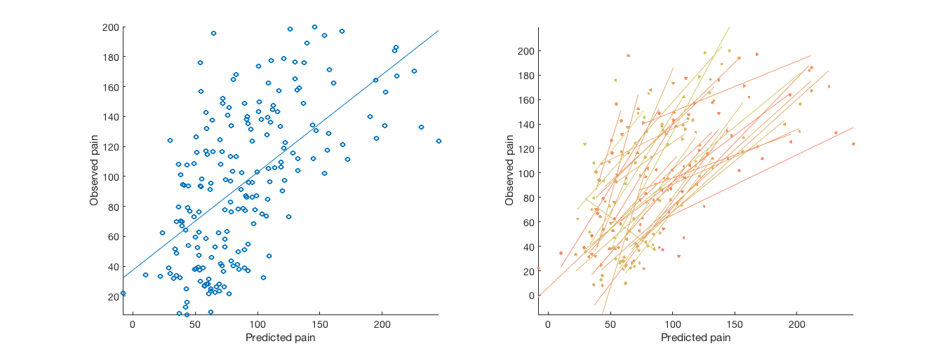
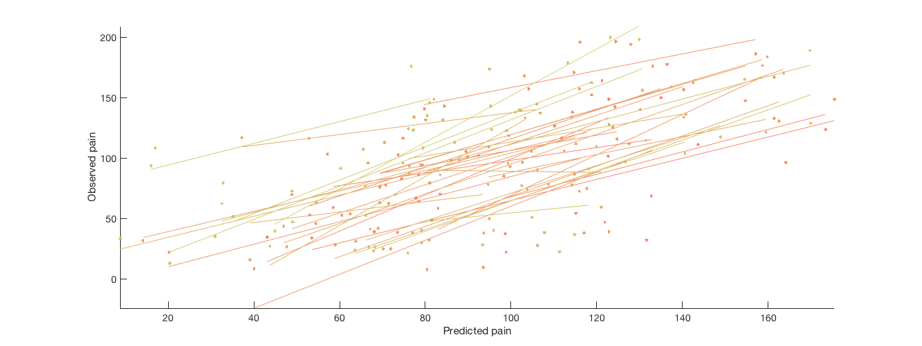
Plot the results
% Plot cross-validated predicted outcomes vs. actual

% Critical fields in stats output structure:
% stats.Y = actual outcomes
% stats.yfit = cross-val predicted outcomes
% pred_outcome_r: Correlation between .yfit and .Y
% weight_obj: Weight map used for prediction (across all subjects).

% Continuous outcomes:

create_figure('scatterplots', 1, 2);
plot(stats.yfit, stats.Y, 'o')
axis tight
refline
xlabel('Predicted pain');
ylabel('Observed pain');

% Consider that each subject has their own line:

for i = 1:n_subjects
    YY{i} = stats.Y(subject_id == i);
    Yfit{i} = stats.yfit(subject_id == i);
end

subplot(1, 2, 2);
line_plot_multisubject(Yfit, YY, 'nofigure');
xlabel('Predicted pain');
ylabel('Observed pain');
axis tight

% Yfit is a cell array, one cell per subject, with fitted values for that subject
average within-person r = 0.60, t( 32) = 7.93, p = 0.000000, num. missing: 0
Summarize within-person classification accuracy
Turn into classification:
% If the stim intensity increases by 1 degree, how often do we correctly
% predict an increase?
diffs = cellfun(@diff, Yfit, 'UniformOutput', false); % successive increases in predicted values with increases in stim intensity

% Subjects (rows) x comparisons (cols), each comparison 1 degree apart
diffs = cat(2, diffs{:})';

acc_per_subject = sum(diffs > 0, 2) ./ size(diffs, 2);
acc_per_comparison = (sum(diffs > 0) ./ size(diffs, 1))';
cohens_d_per_comparison = (mean(diffs) ./ std(diffs))';

fprintf('Mean acc is : %3.2f%% across all successive 1 degree increments\n', 100*mean(acc_per_subject));

% Create and display a table:

comparison = {'45-44' '46-45' '47-46' '48-47' '49-48'}';
results_table = table(comparison, acc_per_comparison, cohens_d_per_comparison);
disp(results_table)

% 45-44 degrees, 46-45, 47-46, etc.
Mean acc is : 73.94% across all successive 1 degree increments
    comparison    acc_per_comparison    cohens_d_per_comparison
    __________    __________________    _______________________

     '45-44'           0.48485                  -0.0587
     '46-45'           0.81818                  0.76512
     '47-46'           0.84848                  0.93114
     '48-47'            0.9697                    1.432
     '49-48'           0.57576                  0.37981
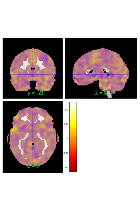
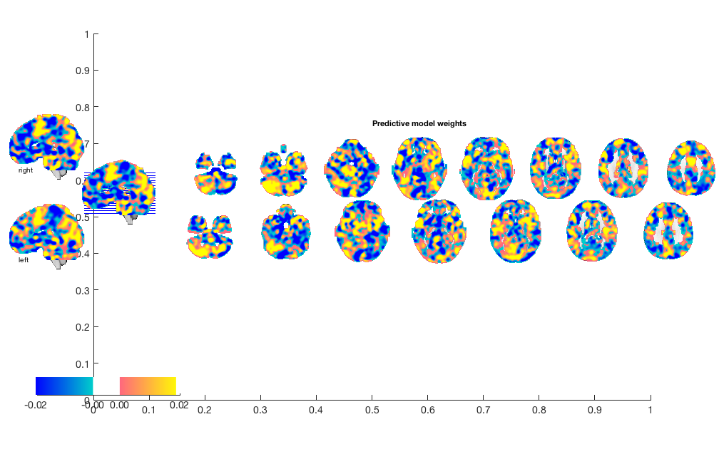
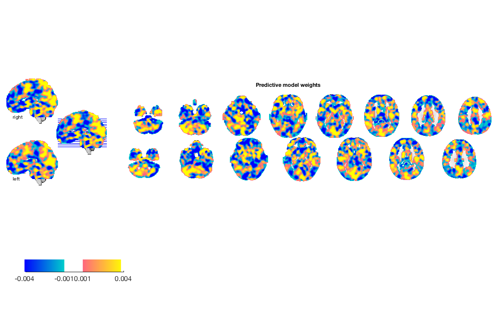
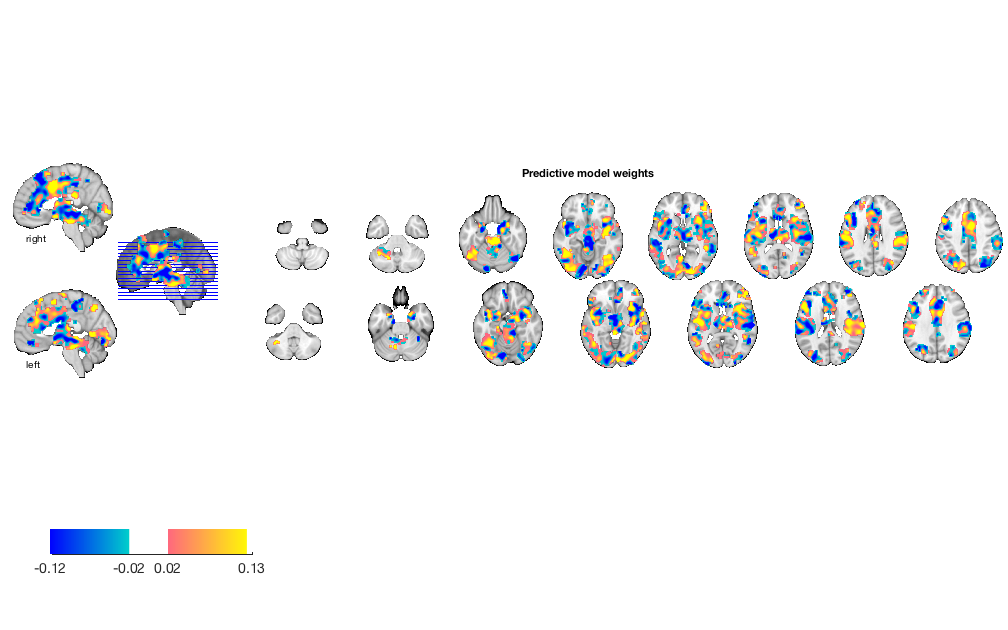
Visualize weight map
w = stats.weight_obj;  % This is an image object that we can view, etc.

orthviews(w)

create_figure('montage');
o2 = montage(w);
o2 = title_montage(o2, 5, 'Predictive model weights');
SPM12: spm_check_registration (v6245)              17:48:58 - 03/08/2018
========================================================================
Display <a href="matlab:spm_image('display','/Users/torwager/Documents/GitHub/CanlabCore/CanlabCore/canlab_canonical_brains/Canonical_brains_surfaces/keuken_2014_enhanced_for_underlay.img,1');">/Users/torwager/Documents/GitHub/CanlabCore/CanlabCore/canlab_canonical_brains/Canonical_brains_surfaces/keuken_2014_enhanced_for_underlay.img,1</a>
Grouping contiguous voxels:   3 regions

ans =

  1×1 cell array

    {1×3 region}

Setting up fmridisplay objects
This takes a lot of memory, and can hang if you have too little.
Grouping contiguous voxels:   3 regions
sagittal montage: 4350 voxels displayed, 219357 not displayed on these slices
sagittal montage: 4292 voxels displayed, 219415 not displayed on these slices
sagittal montage: 3990 voxels displayed, 219717 not displayed on these slices
axial montage: 32223 voxels displayed, 191484 not displayed on these slices
axial montage: 34538 voxels displayed, 189169 not displayed on these slices
Bootstrap weights: Get most reliable weights and p-values for voxels
% Re-run prediction, adding a 'bootstrap' flag.
% For a final analysis, at least 5K bootstrap samples is a good idea

% (This is not run in the example; see help fmri_data.predict for how to
% run bootstrapping)
Try normalizing/scaling data
% z-score every image, removing the mean and dividing by the std.
% Remove some scaling noise, but also some signal...
 image_obj = rescale(image_obj, 'zscoreimages');

% re-run prediction and plot

[cverr, stats, optout] = predict(image_obj, 'algorithm_name', algoname, 'nfolds', holdout_set);

create_figure('scatterplots');

for i = 1:n_subjects
    YY{i} = stats.Y(subject_id == i);
    Yfit{i} = stats.yfit(subject_id == i);
end

line_plot_multisubject(Yfit, YY, 'nofigure');
xlabel('Predicted pain');
ylabel('Observed pain');
axis tight

fprintf('Overall prediction-outcome correlation is %3.2f\n', stats.pred_outcome_r)

figure; o2 = montage(stats.weight_obj);
o2 = title_montage(o2, 5, 'Predictive model weights');
Cross-validated prediction with algorithm cv_lassopcr,   5 folds

Completed fit for all data in:   0 hours   0 min  5 secs
Fold 1/5 done in:   0 hours   0 min  4 sec
Fold 2/5 done in:   0 hours   0 min  3 sec
Fold 3/5 done in:   0 hours   0 min  3 sec
Fold 4/5 done in:   0 hours   0 min  3 sec
Fold 5/5 done in:   0 hours   0 min  4 sec

Total Elapsed Time =   0 hours   0 min 22 sec
average within-person r = 0.59, t( 32) = 13.18, p = 0.000000, num. missing:   0
Overall prediction-outcome correlation is 0.59
Setting up fmridisplay objects
This takes a lot of memory, and can hang if you have too little.
Grouping contiguous voxels:   3 regions
sagittal montage: 4350 voxels displayed, 219357 not displayed on these slices
sagittal montage: 4292 voxels displayed, 219415 not displayed on these slices
sagittal montage: 3990 voxels displayed, 219717 not displayed on these slices
axial montage: 32223 voxels displayed, 191484 not displayed on these slices
axial montage: 34538 voxels displayed, 189169 not displayed on these slices
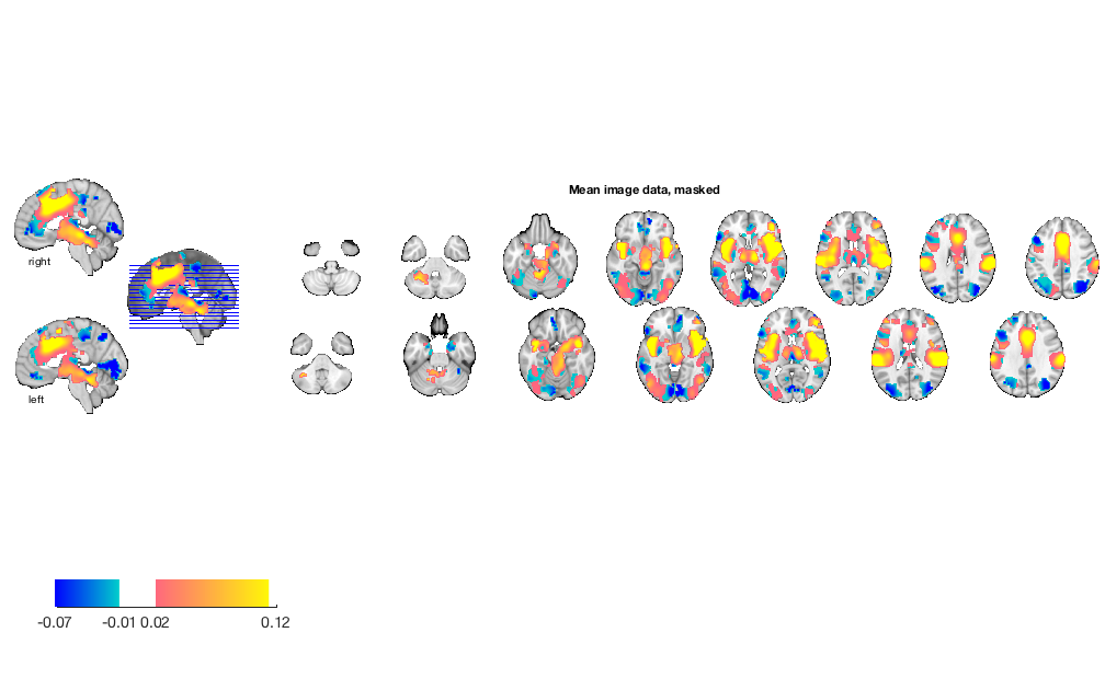
Try selecting an a priori 'network of interest'
% re-load
load('bmrk3_6levels_pain_dataset.mat', 'image_obj')

% load an a priori pain-related mask and apply it

mask = fmri_data(which('pain_2s_z_val_FDR_05.img.gz')); % in Neuroimaging_Pattern_Masks repository

image_obj = apply_mask(image_obj, mask);

% show mean data with mask
m = mean(image_obj);
figure; o2 = montage(m);
o2 = title_montage(o2, 5, 'Mean image data, masked');
Using default mask: /Users/torwager/Documents/GitHub/CanlabCore/CanlabCore/canlab_canonical_brains/Canonical_brains_surfaces/brainmask.nii
loading mask. mapping volumes.
checking that dimensions and voxel sizes of volumes are the same.
Pre-allocating data array. Needed: 1409312 bytes
Loading image number:     1
Elapsed time is 0.019081 seconds.
Image names entered, but fullpath attribute is empty. Getting path info.
Setting up fmridisplay objects
This takes a lot of memory, and can hang if you have too little.
Grouping contiguous voxels:  27 regions
sagittal montage: 1088 voxels displayed, 47895 not displayed on these slices
sagittal montage: 1171 voxels displayed, 47812 not displayed on these slices
sagittal montage: 980 voxels displayed, 48003 not displayed on these slices
axial montage: 7496 voxels displayed, 41487 not displayed on these slices
axial montage: 7950 voxels displayed, 41033 not displayed on these slices
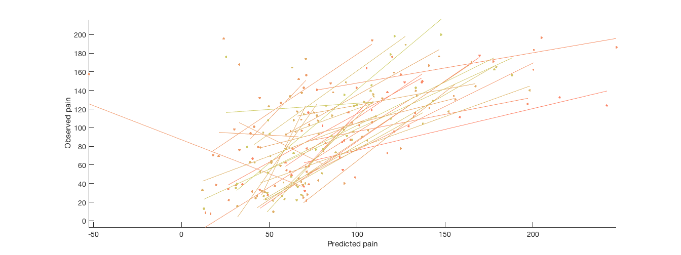
re-run prediction and plot
[cverr, stats, optout] = predict(image_obj, 'algorithm_name', algoname, 'nfolds', holdout_set);

create_figure('scatterplots');

for i = 1:n
    YY{i} = stats.Y(subject_id == i);
    Yfit{i} = stats.yfit(subject_id == i);
end

line_plot_multisubject(Yfit, YY, 'nofigure');
xlabel('Predicted pain');
ylabel('Observed pain');
axis tight

fprintf('Overall prediction-outcome correlation is %3.2f\n', stats.pred_outcome_r)

figure; o2 = montage(stats.weight_obj);
o2 = title_montage(o2, 5, 'Predictive model weights');
Cross-validated prediction with algorithm cv_lassopcr,   5 folds

Completed fit for all data in:   0 hours   0 min  1 secs
Fold 1/5 done in:   0 hours   0 min  1 sec
Fold 2/5 done in:   0 hours   0 min  1 sec
Fold 3/5 done in:   0 hours   0 min  1 sec
Fold 4/5 done in:   0 hours   0 min  1 sec
Fold 5/5 done in:   0 hours   0 min  1 sec

Total Elapsed Time =   0 hours   0 min  4 sec
average within-person r = 0.60, t( 32) = 6.59, p = 0.000000, num. missing:   0
Overall prediction-outcome correlation is 0.60
Setting up fmridisplay objects
This takes a lot of memory, and can hang if you have too little.
Grouping contiguous voxels:  27 regions
sagittal montage: 1088 voxels displayed, 47895 not displayed on these slices
sagittal montage: 1171 voxels displayed, 47812 not displayed on these slices
sagittal montage: 980 voxels displayed, 48003 not displayed on these slices
axial montage: 7496 voxels displayed, 41487 not displayed on these slices
axial montage: 7950 voxels displayed, 41033 not displayed on these slices
Other ideas
There are many ways to build from this basic analysis.
% Data
% ------------
% Examine/clean outliers
% Transformations of data: Scaling/centering to remove global mean,
% ventricle mean
% Identify unaccounted sources of variation/subgroups (experimenter sex,
% etc.)

% Features
% ------------
% A priori regions / meta-analysis
% Feature selection in cross-val loop: Univariate, recursive feature elim