Multi-level kernel density (MKDA) meta-analysis example: Agency database
The starting point for coordinate-based meta-analysis (CBMA) is a text file with the information entered from published studies. In this example, the information is contained in the file "Agency_meta_analysis_database.txt" It is in the Neuroimaging_Pattern_Masks repository on Github.
This file should be on your Matlab path: Neuroimaging_Pattern_Masks/CANlab_Meta_analysis_maps/2011_Agency_Meta_analysis/Agency_meta_analysis_database.txt
Contents
- Section 1: Locate the coordinate database file
- Section 2: Read in and set up the coordinate database
- Check and clean up any variables that need recoding
- Select a subset of contrasts
- Set up and run the analysis
- Reload masked activation map and display slice montage
- Print transparent blobs and activation points on slice montage
- Print table of regions with region labels
- Surface rendering
- Extract and plot study proportion data for significant regions
- Other plots and tables
Dependencies:
% Matlab statistics toolbox
	% Matlab signal processing toolbox
	% Statistical Parametric Mapping (SPM) software https://www.fil.ion.ucl.ac.uk/spm/
	% For full functionality, the full suite of CANlab toolboxes is recommended. See here: Installing Tools
Section 1: Locate the coordinate database file
Also, create a new analysis folder for this analysis
dbfilename = 'Agency_meta_analysis_database.txt';
dbname = which(dbfilename);

if isempty(dbname), error('Cannot locate the file %s\nMake sure it is on your Matlab path.', dbfilename); end

% Create a new directory for the analysis and go there:
analysisdir = fullfile(pwd, 'Agency_meta_analysis_example');
mkdir(analysisdir)
cd(analysisdir)
Section 2: Read in and set up the coordinate database
When you set up your own database, several rules apply. Formatting the spreadsheet so it loads correctly can sometimes be the hardest part of running a meta-analysis.
See https://canlabweb.colorado.edu/wiki/doku.php/help/meta/meta_analysis_mkda
And https://canlabweb.colorado.edu/wiki/doku.php/help/meta/database
Here are some rules for setting up the file: 1 The variable "dbname" in the workspace should specify the name of your coordinate database file 2 The database must be a text file, tab delimited 3 The 1st row of the database must contain the number of columns as its 1st and only entry 4 The 2nd row of database must contain variable names (text, no spaces or special characters) 5 The 3rd - nth rows of the database contains data 6 Talairach coordinates are indicated by T88 in CoordSys variable 7 coordinate fields should be called x, y, and z 8 Do NOT use Z, or any other field name in clusters structure
The second row of your database should contain names for each variable you have coded. Some variables should be named with special keywords, because they are used in the meta-analysis code. Other variables can be named anything, as long as there are no spaces or special characters in the name (e.g., !@#$%^&*(){}[] ~`\/|<>,.?/;:"''+=). Anything that you could not name a variable in Matlab will also not work here. Here are the variable names with special meaning. They are case-sensitive:
Subjects : Sample size of the study to which the coordinate belongs
FixedRandom : Study used fixed or random effects. Values should be Fixed or Random. Fixed effects coordinates will be automatically downweighted
SubjectiveWeights : A coordinate or contrast weighting vector based on FixedRandom and whatever else you want to weight by; e.g., study reporting threshold The default is to use FixedRandom only if available
x, y, z : X, Y, and Z coordinates
study : name of study
Contrast : unique indices (e.g., 1:k) for each independent contrast. This is a required variable! All rows belonging to the same contrast should (almost) always have the same values for every variable other than x, y, and z.
CoordSys : Values should be MNI or T88, for MNI space or Talairach space Talairach coordinates will be converted to MNI using Matthew Brett's transform
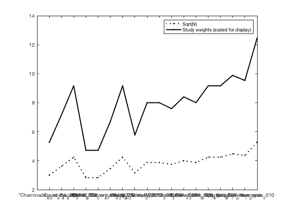
% Read in the database and save it in a structure variable called "DB"
clear DB
read_database;

% Optional: Create SubjectiveWeights
% We will skip this step, but you can use the SubjectiveWeights field to
% assign weights to coordinates. Weights should be between zero and 1


% Prepare the database by checking fields and separating contrasts,
% specifying a 10 mm radius for integrating coordinates:
DB = Meta_Setup(DB, 10);

% Meta_Setup automatically saves a file called SETUP.mat in your folder as well.
drawnow, snapnow
close
Converting T88 coordinates to MNI (M. Brett transform):  12 Transformed
Converting MNI coordinates to T88 for XYZtal array:  34 Transformed
Radius is 10 mm.
Setup. Cannot find Subjects field.  Copying from N.
No xyz field in DB.  Creating from x, y, z.
DB structure saved in SETUP.mat
Contrast image writing is OFF.  Use Meta_Activation_FWE for analysis.
DB struct output of Meta_Setup saved in SETUP.mat
Use info in this file to run next step
Check and clean up any variables that need recoding
This is a good time to examine the DB structure to check whether the variables you entered look as intended (numeric or text), and clean up any variables that need recoding. Sometimes, if text characters are entered in the spreadsheet in a column of numbers, the entire column will be read in as text. Other times, variable entries with the same intended category/level will have different names, e.g., yes vs. Yes (all entries are case-sensitive). You can either fix these in the spreadsheet (best) or re-code them here.
There is no re-coding needed for this dataset, but here is an example: e.g., wh = strcmp(DB.Increased_craving, 'yes'); DB.Increased_craving(wh) = {'Yes'};
% If you do re-code, do this afterwards:
% save SETUP -append DB
Select a subset of contrasts
The function Meta_Select_Contrasts allows you to select a subset of the database (DB variable) based on a combination of selected levels on multiple variables. We will skip that for this example, but if you do select variables, it is a good idea to create a subfolder for the analysis with selected coordinates, and save the DB variable in SETUP.mat in that folder, along with other results you may generate.
Set up and run the analysis
This step prepares the dataset for meta-analysis and runs the entire analysis. It then generates results maps.
It will generate new files for the analysis, so it is a good idea to create and go to a subfolder that will contain files for this analysis. Many meta-analysis projects involve several analyses, in several sub-folders.
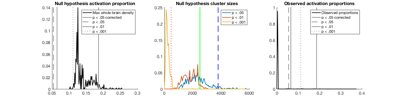
modeldir = fullfile(analysisdir, 'MKDA_all_contrasts');
mkdir(modeldir)
cd(modeldir)

Meta_Activation_FWE('all', DB, 500, 'nocontrasts', 'noverbose');

% Note: For a "final" analysis, 10,000 iterations are recommended
%       Because we typically care about inferences at the "tails" of the
%       sampling distribution (i.e., voxels with low P-values)
%
% Note: You can also use Meta_Activation_FWE to do each piece separately:
%
% Meta_Activation_FWE('setup')          % sets up the analysis
%                                       Convolve with spheres and set up the study indicator dataset
% Meta_Activation_FWE('mc', 10000)      % Adds 10,000 Monte Carlo iterations
%
% A file is saved every 10 iterations, so if there are existing saved iterations
% this will find them and add more.
%
% Meta_Activation_FWE('results')        % generates results maps

drawnow, snapnow
No MC iterations found yet. Creating maxprop, uncor_prop, maxcsize
Elapsed time is 39.192333 seconds.
p <= .05 Corrected: Thresh = 0.1860, 1229 voxels
Writing image: Activation_FWE_height.img
Thresh = 0.1113, size threshold = 482: 4838 sig. voxels.
Cluster sizes range from 1875 to 2963
Writing image: Activation_FWE_extent_stringent.img
Thresh = 0.0645, size threshold = 2512: 4484 sig. voxels.
Cluster sizes range from 4484 to 4484
Writing image: Activation_FWE_extent_medium.img
Thresh = 0.0541, size threshold = 3795: 5559 sig. voxels.
Cluster sizes range from 5559 to 5559
Writing image: Activation_FWE_extent_lenient.img
Writing image: Activation_FWE_extent.img
Writing image: Activation_FWE_all.img
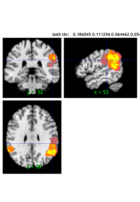
iimg_multi_threshold viewer
=====================================================
Showing positive or negative: both
Overlay is: /Users/torwager/Documents/GitHub/CanlabCore/CanlabCore/canlab_canonical_brains/Canonical_brains_surfaces/SPM8_colin27T1_seg.img
No mask specified in iimg_multi_threshold
Entered p-value image? : No
Height thresholds:0.1860 0.1113 0.0645 0.0541
Extent thresholds: 1 482 2512 3795
Show only contiguous with seed regions: No
SPM12: spm_check_registration (v6245) 23:19:15 - 16/08/2018
========================================================================
Display <a href="matlab:spm_image('display','/Users/torwager/Documents/GitHub/CanlabCore/CanlabCore/canlab_canonical_brains/Canonical_brains_surfaces/SPM8_colin27T1_seg.img,1');">/Users/torwager/Documents/GitHub/CanlabCore/CanlabCore/canlab_canonical_brains/Canonical_brains_surfaces/SPM8_colin27T1_seg.img,1</a>
Saving clusters as cl variable in Activation_clusters.mat
Height
Getting local maxima within 10 mm for subcluster reporting
Z field contains: Unknown statistic (shown in maxstat).
index x y z corr voxels volume_mm3 maxstat
1 52 -52 30 NaN 914 -7312 0.37
-> 52 -52 16 NaN 257 0.31902
-> 50 -58 32 NaN 303 0.36035
-> 54 -50 38 NaN 163 0.37312
-> 56 -40 38 NaN 120 0.29687
-> 52 -56 42 NaN 71 0.35867
2 -52 -52 20 NaN 10 -80 0.23
3 54 -42 24 NaN 1 -8 0.24
4 -58 -52 30 NaN 21 -168 0.22
5 -46 -50 46 NaN 283 -2264 0.35
-> -44 -52 42 NaN 144 0.33780
-> -46 -46 48 NaN 95 0.34903
-> -44 -52 52 NaN 44 0.29317
Additional regions at Extent: Stringent and size >= 10
Z field contains: Unknown statistic (shown in maxstat).
index x y z corr voxels volume_mm3 maxstat
1 -50 -50 36 NaN 1561 -12488 0.18
Additional regions at Extent: Medium and size >= 10
Z field contains: Unknown statistic (shown in maxstat).
index x y z corr voxels volume_mm3 maxstat
1 48 -62 32 NaN 1485 -11880 0.11
2 42 -50 34 NaN 14 -112 0.11
3 62 -34 40 NaN 16 -128 0.11
Additional regions at Extent: Lenient and size >= 10
Z field contains: Unknown statistic (shown in maxstat).
index x y z corr voxels volume_mm3 maxstat
1 54 -32 30 NaN 1068 -8544 0.06
ans =
1×4 cell array
{1×5 struct} {1×2 struct} {1×8 struct} {1×7 struct}
Reload masked activation map and display slice montage
The code below uses the CANlab object-oriented tools, in CANlab_Core_Tools repository. There are many more options for visualization and data analysis
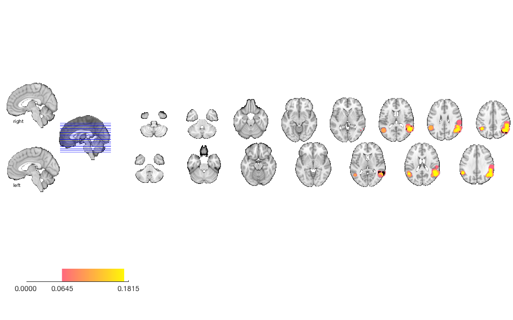
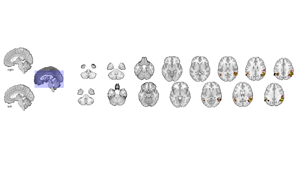
% load saved results mask (union of all thresholds)
img = fmri_data('Activation_FWE_all.img', 'noverbose');  % Create an fmri_data-class object

create_figure('slice montage'); axis off
o2 = montage(img);                                       % Display montage, and return an fmridisplay object called o2

drawnow, snapnow
Setting up fmridisplay objects
This takes a lot of memory, and can hang if you have too little.
Grouping contiguous voxels:   2 regions
sagittal montage:   0 voxels displayed, 7434 not displayed on these slices
sagittal montage:   0 voxels displayed, 7434 not displayed on these slices
sagittal montage:   0 voxels displayed, 7434 not displayed on these slices
axial montage: 1135 voxels displayed, 6299 not displayed on these slices
axial montage: 1176 voxels displayed, 6258 not displayed on these slices
Print transparent blobs and activation points on slice montage
o2 = removeblobs(o2);
o2 = addblobs(o2, r, 'trans', 'transvalue', .4);
o2 = addpoints(o2, DB.xyz, 'MarkerFaceColor', [.5 0 0], 'Marker', 'o', 'MarkerSize', 4);

drawnow, snapnow
sagittal montage:   0 voxels displayed, 7454 not displayed on these slices
sagittal montage:   0 voxels displayed, 7454 not displayed on these slices
sagittal montage:   0 voxels displayed, 7454 not displayed on these slices
axial montage: 1135 voxels displayed, 6319 not displayed on these slices
axial montage: 1182 voxels displayed, 6272 not displayed on these slices
Plotting points within 8.00 mm of slices
Plotting points within 8.00 mm of slices
Plotting points within 8.00 mm of slices
Plotting points within 6.00 mm of slices
Plotting points within 6.00 mm of slices
Print table of regions with region labels
r = region(img);            % Create a region-class object

[rpos, rneg] = table(r);    % Print table, returning regions separated by those with positive or negative data values
                            % Attach names

r = [rpos rneg];            % re-concatenate for convenience later
Grouping contiguous voxels:   2 regions

____________________________________________________________________________________________________________________________________________
Positive Effects
          Region          Volume           XYZ            maxZ      modal_label_descriptions     Perc_covered_by_label    Atlas_regions_covered    region_index
    __________________    ______    _________________    _______    _________________________    _____________________    _____________________    ____________

    'Multiple regions'    44472      52    -50     30    0.37312    'Cortex_Fronto_ParietalB'             14                       12                   1
    'Ctx_PFm_L'           15000     -48    -52     38    0.34904    'Cortex_Fronto_ParietalB'             17                        5                   2


Negative Effects
No regions to display

____________________________________________________________________________________________________________________________________________
Regions labeled by reference atlas CANlab_2018_combined

Volume: Volume of contiguous region in cubic mm.
MaxZ: Signed max over Input mask image values for each voxel.
Atlas_regions_covered: Number of reference atlas regions covered at least 25% by the region. This relates to whether the region covers
multiple reference atlas regions
Region: Best reference atlas label, defined as reference region with highest number of in-region voxels. Regions covering >25% of >5
regions labeled as "Multiple regions"
Perc_covered_by_label: Percentage of the region covered by the label.
Ref_region_perc: Percentage of the label region within the target region.
modal_atlas_index: Index number of label region in reference atlas
all_regions_covered: All regions covered >5% in descending order of importance

For example, if a region is labeled 'TE1a' and Perc_covered_by_label = 8, Ref_region_perc = 38, and Atlas_regions_covered = 17, this means
that 8% of the region's voxels are labeled TE1a, which is the highest percentage among reference label regions. 38% of the region TE1a is
covered by the region. However, the region covers at least 25% of 17 distinct labeled reference regions.

References for atlases:

Beliveau, Vincent, Claus Svarer, Vibe G. Frokjaer, Gitte M. Knudsen, Douglas N. Greve, and Patrick M. Fisher. 2015. “Functional
Connectivity of the Dorsal and Median Raphe Nuclei at Rest.” NeuroImage 116 (August): 187–95.
Bär, Karl-Jürgen, Feliberto de la Cruz, Andy Schumann, Stefanie Koehler, Heinrich Sauer, Hugo Critchley, and Gerd Wagner. 2016. ?Functional
Connectivity and Network Analysis of Midbrain and Brainstem Nuclei.? NeuroImage 134 (July):53?63.
Diedrichsen, Jörn, Joshua H. Balsters, Jonathan Flavell, Emma Cussans, and Narender Ramnani. 2009. A Probabilistic MR Atlas of the Human
Cerebellum. NeuroImage 46 (1): 39?46.
Fairhurst, Merle, Katja Wiech, Paul Dunckley, and Irene Tracey. 2007. ?Anticipatory Brainstem Activity Predicts Neural Processing of Pain
in Humans.? Pain 128 (1-2):101?10.
Fan 2016 Cerebral Cortex; doi:10.1093/cercor/bhw157
Glasser, Matthew F., Timothy S. Coalson, Emma C. Robinson, Carl D. Hacker, John Harwell, Essa Yacoub, Kamil Ugurbil, et al. 2016. A
Multi-Modal Parcellation of Human Cerebral Cortex. Nature 536 (7615): 171?78.
Keren, Noam I., Carl T. Lozar, Kelly C. Harris, Paul S. Morgan, and Mark A. Eckert. 2009. “In Vivo Mapping of the Human Locus Coeruleus.”
NeuroImage 47 (4): 1261–67.
Keuken, M. C., P-L Bazin, L. Crown, J. Hootsmans, A. Laufer, C. Müller-Axt, R. Sier, et al. 2014. “Quantifying Inter-Individual Anatomical
Variability in the Subcortex Using 7 T Structural MRI.” NeuroImage 94 (July): 40–46.
Krauth A, Blanc R, Poveda A, Jeanmonod D, Morel A, Székely G. (2010) A mean three-dimensional atlas of the human thalamus: generation from
multiple histological data. Neuroimage. 2010 Feb 1;49(3):2053-62. Jakab A, Blanc R, Berényi EL, Székely G. (2012) Generation of
Individualized Thalamus Target Maps by Using Statistical Shape Models and Thalamocortical Tractography. AJNR Am J Neuroradiol. 33:
2110-2116, doi: 10.3174/ajnr.A3140
Nash, Paul G., Vaughan G. Macefield, Iven J. Klineberg, Greg M. Murray, and Luke A. Henderson. 2009. ?Differential Activation of the Human
Trigeminal Nuclear Complex by Noxious and Non-Noxious Orofacial Stimulation.? Human Brain Mapping 30 (11):3772?82.
Pauli 2018 Bioarxiv: CIT168 from Human Connectome Project data
Pauli, Wolfgang M., Amanda N. Nili, and J. Michael Tyszka. 2018. ?A High-Resolution Probabilistic in Vivo Atlas of Human Subcortical Brain
Nuclei.? Scientific Data 5 (April): 180063.
Pauli, Wolfgang M., Randall C. O?Reilly, Tal Yarkoni, and Tor D. Wager. 2016. ?Regional Specialization within the Human Striatum for
Diverse Psychological Functions.? Proceedings of the National Academy of Sciences of the United States of America 113 (7): 1907?12.
Sclocco, Roberta, Florian Beissner, Gaelle Desbordes, Jonathan R. Polimeni, Lawrence L. Wald, Norman W. Kettner, Jieun Kim, et al. 2016.
?Neuroimaging Brainstem Circuitry Supporting Cardiovagal Response to Pain: A Combined Heart Rate Variability/ultrahigh-Field (7 T)
Functional Magnetic Resonance Imaging Study.? Philosophical Transactions. Series A, Mathematical, Physical, and Engineering Sciences 374
(2067). rsta.royalsocietypublishing.org. https://doi.org/10.1098/rsta.2015.0189.
Shen, X., F. Tokoglu, X. Papademetris, and R. T. Constable. 2013. “Groupwise Whole-Brain Parcellation from Resting-State fMRI Data for
Network Node Identification.” NeuroImage 82 (November): 403–15.
Zambreanu, L., R. G. Wise, J. C. W. Brooks, G. D. Iannetti, and I. Tracey. 2005. ?A Role for the Brainstem in Central Sensitisation in
Humans. Evidence from Functional Magnetic Resonance Imaging.? Pain 114 (3):397?407.

Note: Region object r(i).title contains full list of reference atlas regions covered by each cluster.
____________________________________________________________________________________________________________________________________________
Surface rendering
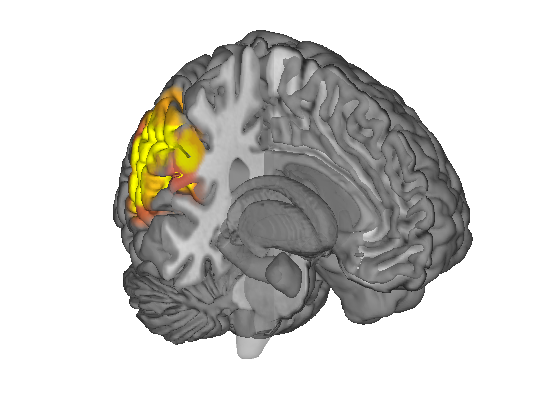
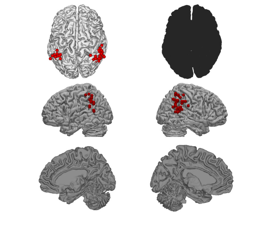
% Create a cutaway surface with blobs
surface(img, 'cutaway', 'ycut_mm', -30);

drawnow, snapnow

% Plot points as spheres on a canonical surface:

plot_points_on_surface2(DB.xyz, {[.5 0 0]});

drawnow, snapnow
Grouping contiguous voxels:   2 regions

ans =

  Light with properties:

       Color: [1 1 1]
       Style: 'infinite'
    Position: [1.4142 -8.6596e-17 0]
     Visible: 'on'

  Use GET to show all properties

Loading structural image: /Users/torwager/Documents/GitHub/CanlabCore/CanlabCore/canlab_canonical_brains/Canonical_brains_surfaces/SPM8_colin27T1_seg.img
Loading image SPM8_colin27T1_seg
    loaded 50 slices
    loaded 100 slices
    loaded 150 slices
Loading structural image: /Users/torwager/Documents/GitHub/CanlabCore/CanlabCore/canlab_canonical_brains/Canonical_brains_surfaces/SPM8_colin27T1_seg.img
Loading image SPM8_colin27T1_seg
    loaded 50 slices
    loaded 100 slices
    loaded 150 slices

ans =

  Light with properties:

       Color: [1 1 1]
       Style: 'infinite'
    Position: [1.0186 0.9498 0.2456]
     Visible: 'on'

  Use GET to show all properties

Using custom color maps.
Found surface patch handles - plotting on existing surfaces.
cluster_surf
___________________________________________
	  1 cluster structures entered
  Colors are:
 1  0  0
 Building XYZ coord list

ans =

  single

   20.0077

 Getting heat-mapped colors
 Building color change function call
 Using existing surface image
 Running color change.
 eval: [c,alld] = getVertexColors(xyz{1},p,mycolors{1},[.5 .5 .5],4,'ovlcolor',[0 1 1],'colorscale',actcolors{1},'alphascale',alphascale{1});
Main color vertices: 864 vertices.  selecting:   0
 eval: [c,alld] = getVertexColors(xyz{1},p,mycolors{1},[.5 .5 .5],4,'ovlcolor',[0 1 1],'colorscale',actcolors{1},'alphascale',alphascale{1});
Main color vertices: 1600 vertices.  selecting:   0
 eval: [c,alld] = getVertexColors(xyz{1},p,mycolors{1},[.5 .5 .5],4,'ovlcolor',[0 1 1],'colorscale',actcolors{1},'alphascale',alphascale{1});
Main color vertices: 1182 vertices.  selecting:  36
7434 coords.  selecting:  eval: [c,alld] = getVertexColors(xyz{1},p,mycolors{1},[.5 .5 .5],4,'ovlcolor',[0 1 1],'colorscale',actcolors{1},'alphascale',alphascale{1});
Main color vertices: 7690 vertices.  selecting: 4172
7434 coords.  selecting:  eval: [c,alld] = getVertexColors(xyz{1},p,mycolors{1},[.5 .5 .5],4,'ovlcolor',[0 1 1],'colorscale',actcolors{1},'alphascale',alphascale{1});
Main color vertices: 1302 vertices.  selecting:   0
 eval: [c,alld] = getVertexColors(xyz{1},p,mycolors{1},[.5 .5 .5],4,'ovlcolor',[0 1 1],'colorscale',actcolors{1},'alphascale',alphascale{1});
Main color vertices: 221348 vertices.  selecting: 55710
7434 coords.  selecting: 1875
Running   2 sets of coordinates: 002 eval: [c,alld] = getVertexColors(xyz{1},p,mycolors{1},[.5 .5 .5],4,'ovlcolor',[0 1 1],'colorscale',actcolors{1},'alphascale',alphascale{1});
Main color vertices: 8690 vertices.  selecting: 2069
7434 coords.  selecting:  eval: [c,alld] = getVertexColors(xyz{1},p,mycolors{1},[.5 .5 .5],4,'ovlcolor',[0 1 1],'colorscale',actcolors{1},'alphascale',alphascale{1});
Main color vertices: 7442 vertices.  selecting: 1034
7434 coords.  selecting:  eval: [c,alld] = getVertexColors(xyz{1},p,mycolors{1},[.5 .5 .5],4,'ovlcolor',[0 1 1],'colorscale',actcolors{1},'alphascale',alphascale{1});
Main color vertices: 2036 vertices.  selecting: 193
7434 coords.  selecting:  eval: [c,alld] = getVertexColors(xyz{1},p,mycolors{1},[.5 .5 .5],4,'ovlcolor',[0 1 1],'colorscale',actcolors{1},'alphascale',alphascale{1});
Main color vertices: 792 vertices.  selecting:  51
7434 coords.  selecting:  eval: [c,alld] = getVertexColors(xyz{1},p,mycolors{1},[.5 .5 .5],4,'ovlcolor',[0 1 1],'colorscale',actcolors{1},'alphascale',alphascale{1});
Main color vertices: 508 vertices.  selecting:   0
 eval: [c,alld] = getVertexColors(xyz{1},p,mycolors{1},[.5 .5 .5],4,'ovlcolor',[0 1 1],'colorscale',actcolors{1},'alphascale',alphascale{1});
Main color vertices: 2734 vertices.  selecting: 312
7434 coords.  selecting:  eval: [c,alld] = getVertexColors(xyz{1},p,mycolors{1},[.5 .5 .5],4,'ovlcolor',[0 1 1],'colorscale',actcolors{1},'alphascale',alphascale{1});
Main color vertices: 193476 vertices.  selecting: 76839
7434 coords.  selecting: 7084
Running   8 sets of coordinates: 008 eval: [c,alld] = getVertexColors(xyz{1},p,mycolors{1},[.5 .5 .5],4,'ovlcolor',[0 1 1],'colorscale',actcolors{1},'alphascale',alphascale{1});
Main color vertices: 13386 vertices.  selecting: 8021
7434 coords.  selecting: 471
Running   1 sets of coordinates: 001 eval: [c,alld] = getVertexColors(xyz{1},p,mycolors{1},[.5 .5 .5],4,'ovlcolor',[0 1 1],'colorscale',actcolors{1},'alphascale',alphascale{1});
Main color vertices: 72554 vertices.  selecting: 10019
7434 coords.  selecting: 1875
Running   2 sets of coordinates: 002 eval: [c,alld] = getVertexColors(xyz{1},p,mycolors{1},[.5 .5 .5],4,'ovlcolor',[0 1 1],'colorscale',actcolors{1},'alphascale',alphascale{1});
Main color vertices: 16841 vertices.  selecting: 4322
7434 coords.  selecting: Finished!
___________________________________________
Using single color for all point classes because you input a single color
Not plotting text codes.
Plotting all peaks; no averaging.
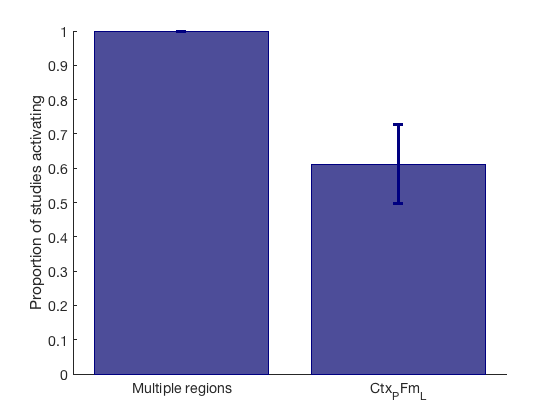
Extract and plot study proportion data for significant regions
First, we will load the MC_Info.mat file, which contains lots of information about the analysis. The variable of main interest in this
% file is MC_Setup, which contains the contrast indicator maps.
% This is stored in MC_Setup.unweighted_study_data

load MC_Info

% MC_Setup =
%     unweighted_study_data: [231202×18 double]             % Voxels x contrast indicator maps (1/0)
%                   volInfo: [1×1 struct]                   % Info for mapping back into brain space
%                         n: [2 3 2 2 1 2 1 2 4 2 2 3 3 2 2 8 2 1] % Coordinates per study
%                       wts: [18×1 double]                  % Contrast weights
%                         r: 5                              % Radius in voxels
%                        cl: {1×18 cell}                    % contiguous blobs for each contrast, for Monte Carlo

indicator_maps = MC_Setup.unweighted_study_data;

% Extract indicator for contrasts that activate within 10 mm (5 vox) of
% significant voxels region object r
[studybyroi,studybyset] = Meta_cluster_tools('getdata', r, indicator_maps, MC_Setup.volInfo);

% studybyroi: contrasts x regions, values 1/0 for whether each contrast activates the region
% studybyset: contrasts x 1, values 1/0 for whether each contrast activates any region in the set

create_figure('Activation_proportions')

[n, k] = size(studybyroi);
prop_by_condition = sum(studybyroi) ./ n;                        % Proportion of contrasts activating each ROI
se = ( (prop_by_condition .* (1-prop_by_condition) ) ./ n ).^.5; % Standard Error based on binomial distribution

han = bar(prop_by_condition);
ehan = errorbar(prop_by_condition, se);

set(han, 'EdgeColor', [0 0 .5], 'FaceColor', [.3 .3 .6]);
set(ehan, 'Color', [0 0 .5], 'LineStyle', 'none', 'LineWidth', 3);
set(gca, 'XTick', 1:k, 'XLim', [.5 k+.5], 'XTickLabel', {r.shorttitle});
ylabel('Proportion of studies activating');
ans =

  Figure (Activation_proportions) with properties:

      Number: 6
        Name: 'Activation_proportions'
       Color: [1 1 1]
    Position: [560 528 560 420]
       Units: 'pixels'

  Use GET to show all properties
Other plots and tables
% Print a table of regions, separating local maxima
% There are other options for other types of tables, separating by
% subpeaks, lateralization, and other things.  We will leave that for later
% walkthroughs.

%tic
%cl = Meta_cluster_tools('make_table', r, MC_Setup, true, false);
%toc

% Another desirable thing to do is to plot and analyze activation
% proportions in region as a function of study conditions (e.g., type of
% study).
% We won't do this here, but to plot a bar plot of ROI counts for different
% conditions, try:
% [prop_by_condition,se,num_by_condition,n] = Meta_cluster_tools('count_by_condition',dat,Xi,w,doplot,[xnames],[seriesnames], [colors])