Linear Mixed Model demo
Contents
This demonstration was prepared by Bogdan Petre and Tor Wager
It includes code to perform a mixed-effects analysis on a dataset in both Matlab and R. The published version runs the Matlab code.
To reproduce the analysis, you must have the dataset, which is in the CANlab_help_examples repository on Github, on your Matlab path. it is in the subfolder canlab_mixed_effects_matlab_demo1
About the dataset
The example uses a subset of data from an ongoing study, provided for model demonstration purposes only. Do not reuse or reshare this dataset for other purposes. It was collected by Tor Wager's Cognitive and Affective Neuroscience lab at the University of Colorado.
behav_dat = readtable('study_behav_dat_sid_14_164.csv');

behav_dat(1:5, :)

% we remove this subject who only has placebo but no contorl data
% glmfit_multilevel isn't designed to handle this
%behav_dat(behav_dat.sid == 113,:) = [];
ans =

  5×11 table

     Yint       Yunp       RTint      RTunp     stimLvl    sid    heat    placebo    run    trial     vif
    _______    _______    _______    _______    _______    ___    ____    _______    ___    _____    ______

    0.91016          1     3.4159     4.4826     -0.5       6      1       -0.5       1     -1.5     2.0965
    0.59766     0.4668     3.6492     2.5496      0.5       6      1       -0.5       1     -0.5     1.7078
          0          0    0.81655    0.68308     -0.5       6      1       -0.5       1      0.5     1.7062
          0          0    0.46561    0.46575     -0.5       6      0       -0.5       1     -0.5     1.4626
    0.82031    0.55664      3.466     3.3659      0.5       6      0       -0.5       1      0.5     1.5805
*Variables*
% Yint - pain intensity rating
% Yunp - pain unpleasantness rating.
% RTint - reaction time for intensity ratings
% RTunp - reaction time for unpleasantness ratings
% stimLvl - low, medium or high. 46.5C, 47C and 47.5C, possibly different
%   for earliest subjects, but we think all with different temps are excluded
% sid - subject id label. Corresponds to PGsXXX labels used internally by
%   the lab
% heat - 1 if heat trial, 0 for pressure trials
% placebo - 0.5 for stimulation of placebo treated sight, -0.5
%   otherwise
% run - run number(1,2,3 or 4). Runs 1 and 4 are ctrl. 2 and 3 are
%   placebo.
% trial - trial number within run. Centered.
% vif - variance inflation factor for use with fMRI data. can ignore this.
*Preparation*
% this data was prepared with various preprocessing steps:
% any response times <= 0.02s were removed (we had sticky button problems
%   and based on temporal distribution of responses it seems that anything
%   < 0.02 is likely to be due to this rather than a deliberate response)
% any response times >= 5.01 seconds. These are timeouts without a click
%   and it's ambiguous whether the cursor location recorded corresponds to
%   the subjects rating or not.
% subjects with sid 1-13 were removed due to changes to the paradigm at
%   this stage of the study. Subject 6 retained because this subject was
%   processed out of order and actually was run on the newer paradigm.
% subject 23 and 84 are removed because too few of their responses passed
%   the timing criteria above
Using fitlme to create a LinearMixedModel object in Matlab
The fitlme code below does the following:
% - test placebo effect on heat trials
% - Control for stimulus level and test for interaction effects.
% - Model random subject (sid) intercepts and slopes.
% - Intercept is modeled implicitly both at the group and subject level.
% That is, you do not need to enter 'Yint ~ 1 + stimLvl*placebo ...'
% in the model in order for it to include an intercept term, because fitlme
% adds it automatically.
% - Use REML estimator instead of the default ML.


heat_dat = behav_dat(behav_dat.heat == 1,:); % Use heat trials only

m = fitlme(heat_dat, 'Yint ~ stimLvl*placebo + (stimLvl*placebo | sid)',...
    'FitMethod','REML');
Other notes:
% - Adding stimLvl*placebo automatically adds stimLvl, placebo, and
% stimLvl*placebo effects. You do not need to enter
% 'Yint ~ 1 + stimLvl + placebo + stimLvl*placebo ...'
% 'Yint ~ stimLvl*placebo ...' does the same thing.
%
% - Adding (stimLvl*placebo | sid) adds random effects for the intercept
% (1), added automatically if another random effect is added), stimLvl,
% placebo, and stimLvl*placebo effects.
*Sample output* Here is a sample of the output.
% - The P-values for Fixed effects coefficients do not generalize across
% levels of the random factors. The df and P-values use the overall number
% of observations (1704) minus the number of fixed-effect parameters (4 =
% 1 (intercept) + 1 (stimLvl) + 1 (placebo) + 1 (stimLvl*placebo).
% This is not correct for an inference across levels of the random effect
% of subject (sid).
% Thus, we need to use the anova() function below to get the correct
% inferences.

% Fixed effects coefficients (95% CIs):
%     Name                        Estimate     SE           tStat      DF      pValue        Lower        Upper
%     '(Intercept)'                 0.16402     0.011235     14.598    1700    1.4571e-45      0.14198      0.18606
%     'stimLvl'                    0.073984    0.0091767     8.0622    1700    1.3994e-15     0.055985     0.091983
%     'placebo'                -0.054471    0.0086796    -6.2757    1700    4.4069e-10    -0.071495    -0.037447
%     'stimLvl:placebo'        0.0065812     0.014501    0.45385    1700       0.64999     -0.02186     0.035022
%
% Random effects covariance parameters (95% CIs):
% Group: sid (121 Levels)
%     Name1                       Name2                       Type          Estimate      Lower        Upper
%     '(Intercept)'               '(Intercept)'               'std'            0.11924      0.10469     0.13581
%     'stimLvl'                   '(Intercept)'               'corr'            0.7489      0.71099     0.78247
inspect model coefficients (ignore p-values)
m.Coefficients
ans =


    FIXED EFFECT COEFFICIENTS: DFMETHOD = 'RESIDUAL', ALPHA = 0.05

    Name                       Estimate     SE           tStat      DF
    {'(Intercept)'    }          0.16402     0.011235     14.598    1700
    {'stimLvl'        }         0.073984    0.0091767     8.0622    1700
    {'placebo'        }        -0.054471    0.0086796    -6.2757    1700
    {'stimLvl:placebo'}        0.0065812     0.014501    0.45385    1700


    pValue        Lower        Upper
    1.4571e-45      0.14198      0.18606
    1.3994e-15     0.055985     0.091983
    4.4069e-10    -0.071495    -0.037447
       0.64999     -0.02186     0.035022
get satterthwaite corrected p-values LinearMixedModel.anova Perform hypothesis tests on fixed effect terms. STATS = anova(LME) tests the significance of each fixed effect term in the linear mixed effects model LME and returns a table array STATS. If DummyVarCoding is used in fitlme call, anova will perform Type III hypothesis tests across DummyVar (not shown here).
anova(m,'dfmethod','satterthwaite')
ans =


    ANOVA MARGINAL TESTS: DFMETHOD = 'SATTERTHWAITE'

    Term                       FStat      DF1    DF2       pValue
    {'(Intercept)'    }         213.11    1      120.31    2.1189e-28
    {'stimLvl'        }         64.999    1      127.14     4.762e-13
    {'placebo'        }         39.384    1      121.44    5.5834e-09
    {'stimLvl:placebo'}        0.20598    1      255.48       0.65032
Satterthwaite corrected p-values can also be obtained using LinearMixedModel/coefTest, which can be useful for certain circumstances where anova doesn't return the specific contrast of interest by default. One circumstance where this arises is when you have DummyVarCoding in your fitlme invocation, but it's also useful for performing post-hoc comparisons.
The following implementation tests stimLvl = 0, which should provide the same results as above, while the other should post-hoc test whether placebo + stimLvl = 0, which conceptually amounts to testing if placebo effects are larger than a 1C decrease in stimulus intensity. The test is somewhat contrived, but mostly selected to illustrate how to use coefTest.
[Pa, Fa, DF1a, DF2a] = coefTest(m,[0,1,0,0],0,'dfmethod','satterthwaite');

[Pb, Fb, DF1b, DF2b] = coefTest(m,[0,1,1,0],0,'dfmethod','satterthwaite');

t = array2table([Pa,Fa,DF1a,DF2a; Pb, Fb, DF1b, DF2b],'VariableNames',...
    {'pValue','F','DF1','DF2'},'RowNames',{'stimLvl','placebo = (-1)*stimLvl'})
t =

  2×4 table

                               pValue        F       DF1     DF2
                              _________    ______    ___    ______

    stimLvl                   4.762e-13    64.999     1     127.14
    placebo = (-1)*stimLvl      0.12765    2.3542     1     116.79
*Satterthwaite correction*
% Using the satterthwaite option for df estimates the error degrees of
% freedom based on the rank
% The formula was developed by the statistician Franklin E. Satterthwaite and a derivation of the
% result is given in Satterthwaite's article in Psychometrika (vol. 6, no. 5, October 1941).
% This site is useful for deriving the df in the two-sample case: https://secure-media.collegeboard.org/apc/ap05_stats_allwood_fin4prod.pdf
% Code for Satterthwaite df calculation for mulitple regression can be found in
% fit_gls.m (Martin Lindquist), and is included here for the
% no-autocorrelation (AR(p), p==0) case:

% A = W;   % for ar p = 0 case; weights
% R = (eye(T) - X * invxvx * X' * iV);        % Residual inducing matrix
%
% Wd = R * A * inv(iV) * A';                  % inv(iV) = Covariance matrix
% df = (trace(Wd).^2)./trace(Wd*Wd);       % Satterthwaite approximation for degrees of freedom
*Model properties* You can query the model object (m) to get its properties. e.g.,
help LinearMixedModel
m.Rsquared
m.VariableInfo                          % all variables in input dataset and which are in model
m.Variables(1:5, :)                     % all variables in input dataset
X = designMatrix(m); X(1:5, :)          % Fixed-effects design matrix
Xg = designMatrix(m, 'Random'); whos('Xg')          % Random-effects design matrix


% This option,  'DummyVarCoding', 'effects', effects-codes, which we
% prefer:
m = fitlme(heat_dat,'Yint ~ stimLvl*placebo + (stimLvl*placebo | sid)',...
    'FitMethod','REML', 'DummyVarCoding', 'effects');
% help anova says:
%     To obtain tests for the Type III hypotheses, set the 'DummyVarCoding'
%     to 'effects' when fitting the model.
 LinearMixedModel Fitted linear mixed effects model.
    LME = FITLME(...) fits a linear mixed effects model to data. The fitted
    model LME is a LinearMixedModel modeling a response variable as a
    linear function of fixed effect predictors and random effect
    predictors.

    LinearMixedModel methods:
        coefCI - Coefficient confidence intervals
        coefTest - Linear hypothesis test on coefficients
        predict - Compute predicted values given predictor values
        random - Generate random response values given predictor values
        plotResiduals - Plot of residuals
        designMatrix - Fixed and random effects design matrices
        fixedEffects - Stats on fixed effects
        randomEffects - Stats on random effects
        covarianceParameters - Stats on covariance parameters
        fitted - Fitted response
        residuals - Various types of residuals
        response - Response used to fit the model
        compare - Compare fitted models
        anova - Marginal tests for fixed effect terms
        disp - Display a fitted model

    LinearMixedModel properties:
        FitMethod - Method used for fitting (either 'ML' or 'REML')
        MSE - Mean squared error (estimate of residual variance)
        Formula - Representation of the model used in this fit
        LogLikelihood - Log of likelihood function at coefficient estimates
        DFE - Degrees of freedom for residuals
        SSE - Error sum of squares
        SST - Total sum of squares
        SSR - Regression sum of squares
        CoefficientCovariance - Covariance matrix for coefficient estimates
        CoefficientNames - Coefficient names
        NumCoefficients - Number of coefficients
        NumEstimatedCoefficients - Number of estimated coefficients
        Coefficients - Coefficients and related statistics
        Rsquared - R-squared and adjusted R-squared
        ModelCriterion - AIC and other model criteria
        VariableInfo - Information about variables used in the fit
        ObservationInfo - Information about observations used in the fit
        Variables - Table of variables used in fit
        NumVariables - Number of variables used in fit
        VariableNames - Names of variables used in fit
        NumPredictors - Number of predictors
        PredictorNames - Names of predictors
        ResponseName - Name of response
        NumObservations - Number of observations in the fit
        ObservationNames - Names of observations in the fit

    See also FITLME, FITLMEMATRIX, LinearModel, GeneralizedLinearModel, NonLinearModel.


ans =

  struct with fields:

    Ordinary: 0.5735
    Adjusted: 0.5728


ans =

  11×4 table

                 Class          Range        InModel    IsCategorical
               __________    ____________    _______    _____________

    Yint       {'double'}    {1×2 double}     false         false
    Yunp       {'double'}    {1×2 double}     false         false
    RTint      {'double'}    {1×2 double}     false         false
    RTunp      {'double'}    {1×2 double}     false         false
    stimLvl    {'double'}    {1×2 double}     true          false
    sid        {'double'}    {1×2 double}     true          false
    heat       {'double'}    {1×2 double}     false         false
    placebo    {'double'}    {1×2 double}     true          false
    run        {'double'}    {1×2 double}     false         false
    trial      {'double'}    {1×2 double}     false         false
    vif        {'double'}    {1×2 double}     false         false


ans =

  5×11 table

     Yint       Yunp       RTint      RTunp     stimLvl    sid    heat    placebo    run    trial     vif
    _______    _______    _______    _______    _______    ___    ____    _______    ___    _____    ______

    0.91016          1     3.4159     4.4826     -0.5       6      1       -0.5       1     -1.5     2.0965
    0.59766     0.4668     3.6492     2.5496      0.5       6      1       -0.5       1     -0.5     1.7078
          0          0    0.81655    0.68308     -0.5       6      1       -0.5       1      0.5     1.7062
    0.67578    0.74805     2.0656     4.0154      0.5       6      1        0.5       2     -0.5     1.8016
    0.24609    0.13672     1.3997     1.6329     -0.5       6      1        0.5       2      0.5     1.7161


ans =

    1.0000   -0.5000   -0.5000    0.2500
    1.0000    0.5000   -0.5000   -0.2500
    1.0000   -0.5000   -0.5000    0.2500
    1.0000    0.5000    0.5000    0.2500
    1.0000   -0.5000    0.5000   -0.2500

  Name         Size             Bytes  Class     Attributes

  Xg        1704x484            98472  double    sparse
Simple two-level mixed effects using CANlab glmfit_multilevel
Mixed-effects models differ in their assumptions and implementation details. glmfit_multilevel is a fast and simple option for running a two-level mixed effects model with participant as a random effect. It implements a random-intercept, random-slope model across 2nd-level units (e.g., participants). it fits regressions for individual 2nd-level units (e.g., participants), and then (optionally) uses a precision-weighted least squares approach to model group effects. It thus treats participants as a random effect. This is appropriate when 2nd-level units are participants and 1st-level units are observations (e.g., trials) within participants. glmfit_multilevel was designed with this use case in mind.
glmfit_multilevel requires enough 1st-level units to fit a separate model for each 2nd-level unit (participant). If this is not the case, other models (igls.m, LMER, etc.) are preferred.
Degrees of freedom: glmfit_multilevel is conservative in the sense that the degrees of freedom in the group statistical test is always based on the number of subjects - 2nd-level parameters. The df is never higher than the sample size, which you would have with mixed effects models that estimate the df from the data. This causes problems in many other packages, particularly when there are many 1st-level observations and they are uncorrelated, resulting in large and undesirable estimated df.
% update appropriately
addpath(genpath(['/home/' getenv('USER') '/.matlab/canlab/CanlabCore']));

% provides glmfit_multilevel() dependency RB_empirical_bayes_params()
addpath(genpath(['/home/' getenv('USER') '/.matlab/canlab/MediationToolbox']));
Warning: Function vecnorm has the same name as a MATLAB builtin. We suggest you
rename the function to avoid a potential name conflict.
Warning: Function vecnorm has the same name as a MATLAB builtin. We suggest you
rename the function to avoid a potential name conflict.
Prepare the dataset** glmfit_multilevel takes cell array input, with one cell per subject Y contains the response for each subject, and X the within-subject design matrix.
First, we need to turn the dataset into cell arrays:
u = unique(heat_dat.sid);
[Y, X] = deal(cell(1, length(u)));

Y_name = 'Yint';
X_var_names = {'stimLvl' 'placebo'};

Y_var = heat_dat.(Y_name);

X_var = zeros(size(Y_var, 1), length(X_var_names));

for j = 1:length(X_var_names)
    X_var(:, j) = heat_dat.(X_var_names{j});
end

for i = 1:length(u)

    wh = heat_dat.sid == u(i);  % indicator for this subject

    Y{i} = Y_var(wh);

    for j = 1:length(X_var_names)

        X{i}(:, j) = X_var(wh, j);

    end

end

% X2 is the 2nd-level (between-person) design matrix.
% we don't have any between-person predictors, so X2 is empty here:
X2 = [];

X2_names = {'2nd-level Intercept (average within-person effects)'};
*Between-person predictors* Note: if we had a between-person predictor, the intercept would be first, and names would be, e.g., X2_names = {'2nd-level Intercept (overall group effect)' '2nd-lev predictor: Group membership'}
*Within-person variation* glmfit_multilevel takes a summary statistics approach with precision-reweighting. it fits a model for each person individually. Therefore, each individual must have variance in Y and individual X.
Run the model
stats = glmfit_multilevel(Y, X, X2, 'names', X_var_names, 'beta_names', X2_names);

% The 'weighted' option uses Empirical Bayes weighting for a single-step
% precision reweighting. This is a simple version of what is acccomplished
% by fitlme in Matlab or LMER in R, or igls.m (Lindquist/Wager).

stats = glmfit_multilevel(Y, X, X2, 'names', X_var_names, 'beta_names', X2_names, 'weighted');

% The 'boot' option, with 'bootsamples', n, runs n boostrap samples at the 2nd level:
% Run with 1000 bootstrap samples initially, and more are added based on P-value tolerance to avoid instability with too-few samples

stats = glmfit_multilevel(Y, X, X2, 'names', X_var_names, 'beta_names', X2_names, 'weighted', 'boot');
Warning! Some participants have no variance in X column(s) and will be excluded
Participant numbers:80
Analysis description: Second Level of Multilevel Model
GLS analysis

Observations: 120, Predictors:   1
Outcome names: Intercept	stimLvl	placebo
Weighting option: unweighted
Inference option: t-test

Other Options:
	Plots: No
	Robust: no
	Save: No
	Output file: glmfit_general_output.txt
	Total time: 0.00 s

________________________________________

Second Level of Multilevel Model
	Outcome variables:
	Intercept	stimLvl	placebo
Adj. mean	0.16	0.07	-0.05

2nd-level Intercept (average within-person effects)
	Intercept	stimLvl	placebo
Coeff	0.16	0.07	-0.05
STE	0.01	0.01	0.01
t	14.53	8.23	-6.31
Z	8.21	7.30	-5.85
p	0.00000	0.00000	0.00000

________________________________________
Warning! Some participants have no variance in X column(s) and will be excluded
Participant numbers:80
Analysis description: Second Level of Multilevel Model
GLS analysis

Observations: 120, Predictors:   1
Outcome names: Intercept	stimLvl	placebo
Weighting option: weighted
Inference option: t-test

Other Options:
	Plots: No
	Robust: no
	Save: No
	Output file: glmfit_general_output.txt
	R & B - type Empirical Bayes reweighting.
Total time: 0.01 s

________________________________________

Second Level of Multilevel Model
	Outcome variables:
	Intercept	stimLvl	placebo
Adj. mean	0.16	0.05	-0.05

2nd-level Intercept (average within-person effects)
	Intercept	stimLvl	placebo
Coeff	0.16	0.05	-0.05
STE	0.01	0.01	0.01
t	14.24	6.69	-5.52
Z	8.21	6.11	-5.18
p	0.00000	0.00000	0.00000

________________________________________
Warning! Some participants have no variance in X column(s) and will be excluded
Participant numbers:80
Analysis description: Second Level of Multilevel Model
GLS analysis

Observations: 120, Predictors:   1
Outcome names: Intercept	stimLvl	placebo
Weighting option: weighted
Inference option: bootstrap

Other Options:
	Plots: No
	Robust: no
	Save: No
	Output file: glmfit_general_output.txt
	R & B - type Empirical Bayes reweighting.
 Min p-value is 0.000000. Needed: 5867 samples
 Bootstrapping 5867 samples... Bootstrap done in 0.01 s, bias correct in 0.00 s
Total time: 0.25 s

________________________________________
Average p-value tolerance (average max alpha): 0.0060

Bootstrapped statistics. Bootstrap inference
	Outcome variables:
	Intercept	stimLvl	placebo
Adj. mean	0.16	0.05	-0.05

2nd-level Intercept (average within-person effects)
	Intercept	stimLvl	placebo
Coeff	0.16	0.05	-0.05
STE	0.01	0.01	0.01
t	14.24	6.69	-5.52
Z	3.73	3.77	-3.32
p	0.00019	0.00016	0.00091

________________________________________
Plotting data and effects
This is a crucial part of the analysis process!
with glmfit_multilevel, the 'plots' option generates some plots. you can also use functions including barplot_columns() to plot summary 2nd-level stats, and lineplot_multisubject() to plot individual and group within-person effects
% % stats = glmfit_multilevel(Y, X, X2, 'names', X_var_names, 'beta_names', X2_names, 'weighted', 'boot', 'plots');

effectcolors = {[.5 .5 .5] [.7 .4 .4] [.4 .4 .7]};
Plot the individual within-person effect scores and group summary statistics Note: P values and Cohen's d from the barplot_columns output may not match your model results in stats exactly, because it provides a simple t-test on each column. so you should prefer the stats from the mixed model output.
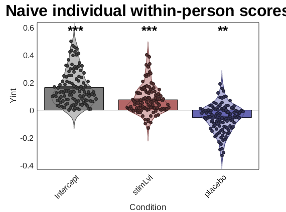
create_figure('2nd level stats');
barplot_columns(stats.first_level.beta', 'names', stats.inputOptions.names, 'colors', effectcolors, 'nofigure');
ylabel(Y_name);
title('Naive individual within-person scores');
drawnow, snapnow
Col   1: Intercept	Col   2: stimLvl	Col   3: placebo
---------------------------------------------
Tests of column means against zero
---------------------------------------------
        Name         Mean_Value    Std_Error      T           P         Cohens_d
    _____________    __________    _________    ______    __________    ________

    {'Intercept'}      0.16386      0.011276    14.532    2.2204e-15      1.3266
    {'stimLvl'  }     0.074936     0.0091093    8.2263    2.7751e-13     0.75096
    {'placebo'  }    -0.054998     0.0087174    -6.309    4.9825e-09    -0.57593
If you are using subject scores on within-person effects for other purposes, e.g., to regress on brain variables, then using the Empirical Bayes estimates for these is a good idea!! They are likely to be more accurate representation of the individual participants' scores than the naive within-person effects.
create_figure('2nd level stats comparison', 1, 2);
subplot(1, 2, 1);
barplot_columns(stats.first_level.beta', 'names', stats.inputOptions.names, 'colors', effectcolors, 'nofigure');
ylabel(Y_name);
title('Naive individual within-person scores');

subplot(1, 2, 2);
barplot_columns(stats.Y_star, 'names', stats.inputOptions.names, 'colors', effectcolors, 'nofigure');
ylabel(Y_name);
title('Empirical Bayes individual scores');
drawnow, snapnow
Col   1: Intercept	Col   2: stimLvl	Col   3: placebo
---------------------------------------------
Tests of column means against zero
---------------------------------------------
        Name         Mean_Value    Std_Error      T           P         Cohens_d
    _____________    __________    _________    ______    __________    ________

    {'Intercept'}      0.16386      0.011276    14.532    2.2204e-15      1.3266
    {'stimLvl'  }     0.074936     0.0091093    8.2263    2.7751e-13     0.75096
    {'placebo'  }    -0.054998     0.0087174    -6.309    4.9825e-09    -0.57593

Col   1: Intercept	Col   2: stimLvl	Col   3: placebo
---------------------------------------------
Tests of column means against zero
---------------------------------------------
        Name         Mean_Value    Std_Error       T           P         Cohens_d
    _____________    __________    _________    _______    __________    ________

    {'Intercept'}      0.15939      0.010343      15.41    2.2204e-15     1.4067
    {'stimLvl'  }     0.067031     0.0058821     11.396    2.2204e-15     1.0403
    {'placebo'  }     -0.05237     0.0062338    -8.4009    1.0938e-13    -0.7669
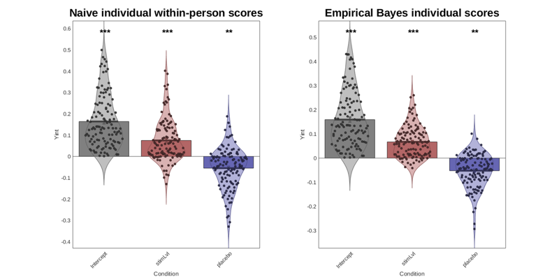
With line_plot_multisubject, you can plot the within-person scores for one effect at a time. This does not control for other effects, and stats reported are simple summary stats, so you should prefer the stats from the mixed model output.
Get one column of X (Alternatively, you could reconstruct individual scores for marginal estimates for each level, or modify glmfit_multilevel to return this output!)
X_placebo = X;
for i = 1:length(X), X_placebo{i} = X_placebo{i}(:, 2); end

%
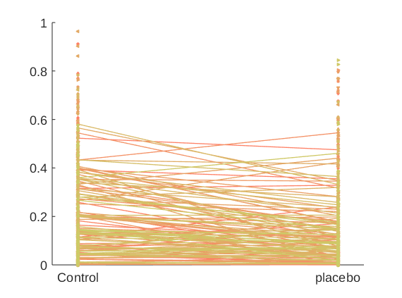
Create a plot, with each subject in a different color along a spectrum
create_figure('1st level effect');
line_plot_multisubject(X_placebo, Y);
set(gca, 'XTick', [-.5 .5], 'XLim', [-.6 .6], 'XTickLabel', {'Control' 'placebo'});
Warnings:

____________________________________________________________________________________________________________________________________________
X: some input cells have no varability:
80
X: input cells with low varability:
80
Y: input cells with low varability:
18 25 53 70 113 116
Excluded some subjects from individual fits:
80
____________________________________________________________________________________________________________________________________________

____________________________________________________________________________________________________________________________________________
Input data:
X scaling: Centered
Y scaling: No centering or z-scoring

Transformations:
No data transformations before plot

Correlations:
r = -0.15 across all observations, based on untransformed input data

Stats on slopes after transformation, subject is random effect:
Mean b = -0.06, t(119) = -6.62, p = 0.000000, num. missing:   1

Average within-person r = -0.21 +- 0.35 (std)

Between-person r (across subject means) = 0.05, p = 0.554204
____________________________________________________________________________________________________________________________________________
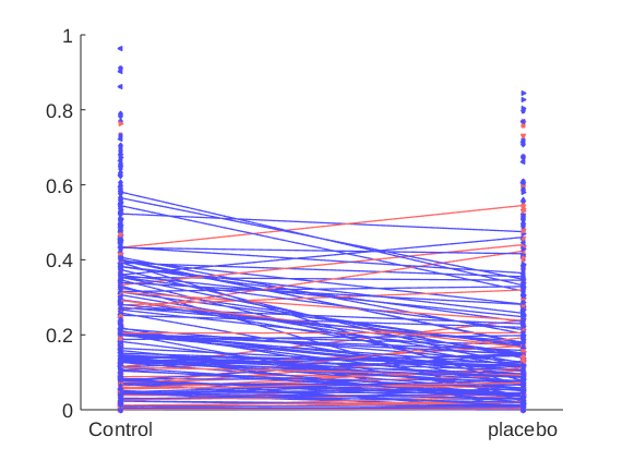
Create a plot with individuals that show positive effects in one color and negative effects in another color (Negative effects mean analgesia here)
indiv_scores = stats.Y_star(:, 3);
% or: indiv_scores = stats.first_level.beta(3, :)';

wh = indiv_scores > 0; % individuals with positive effects

poscolors = {[1 .4 .4]}; % custom_colors([.3 .3 .7], [.3 .5 1], sum(wh))';    % colors for those with pos effects
negcolors = {[.3 .3 1]}; % custom_colors([.7 .2 .2], [.7 .4 .4], sum(~wh))';    % colors for everyone else

colors = {};
colors(wh) = poscolors;
colors(~wh) = negcolors;

create_figure('1st level effect');
line_plot_multisubject(X_placebo, Y, 'colors', colors);
set(gca, 'XTick', [-.5 .5], 'XLim', [-.6 .6], 'XTickLabel', {'Control' 'placebo'});
Warnings:

____________________________________________________________________________________________________________________________________________
X: some input cells have no varability:
80
X: input cells with low varability:
80
Y: input cells with low varability:
18 25 53 70 113 116
Excluded some subjects from individual fits:
80
____________________________________________________________________________________________________________________________________________

____________________________________________________________________________________________________________________________________________
Input data:
X scaling: Centered
Y scaling: No centering or z-scoring

Transformations:
No data transformations before plot

Correlations:
r = -0.15 across all observations, based on untransformed input data

Stats on slopes after transformation, subject is random effect:
Mean b = -0.06, t(119) = -6.62, p = 0.000000, num. missing:   1

Average within-person r = -0.21 +- 0.35 (std)

Between-person r (across subject means) = 0.05, p = 0.554204
____________________________________________________________________________________________________________________________________________
Assessing and considering correlations between the individual effects
Individuals with high stimulus responses might also show large analgesia effects
Or, commonly, the individuals with higher baseline outcomes (here, pain) might show larger effects. This is likely if there are individual differences in the *scale* of the outcome, such that some individuals have compressed values on the outcome relative to others, causing a proportional compression of the treatment effects. This is very common with outcome measures including self-reported symptoms and reaction times. If so, it's ambiguous what the best individual difference scores for treatment effects ought to be. They could be the effect scores in raw units, or after adjusting for potential response scale differences.
In both these cases, the within-person effects will be correlated -- across treatment effects, in the former case, and with the intercept (average outcome value) in the latter. We can assess these empirically, using the EB estimates from our mixed-effects model:
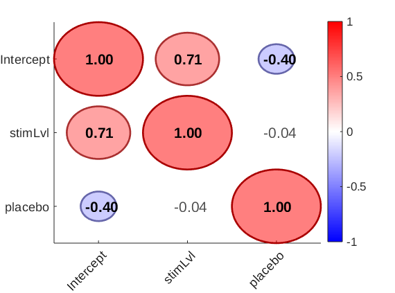
plot_correlation_matrix(stats.Y_star, 'names', stats.inputOptions.names);
drawnow, snapnow
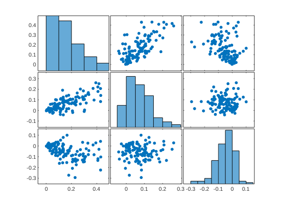
it's also a good idea to look at the scatterplots and marginal distributions (e.g., check for outliers)
figure; plotmatrix(stats.Y_star);
drawnow, snapnow
Here, we see that the intercept (average pain) is strongly correlated with the effect of stimLvl (intensity sensitivity) and also correlated with the effect of placebo (negatively, which is sensible as a negative effect means a larger analgesic effect). This suggests that there are individual differences in scale usage (compressed vs. expanded range) that influence the treatment effect scores when analyzed in raw units. Specifically, e.g., here about half the variation in stimulus intensity effects can be explained by overall pain report differences (r = 0.71)
This can add noise variability that masks effects (makes them non-significant) in the linear model, or when correlating with external variables (e.g., fMRI activity, another task). Or it can create artifactual positive correlations with other tasks (e.g., a different drug/treatment effect) if participants display the same scale compression/expansion across tasks. That is, we might observe positive correlations between placebo effects in pain and in a different task (allergy test) that could be caused by consistency in scale usage rather than consistency in the underlying treatment effects.
Some options for dealing with this include: 1. Include baseline scale (e.g., average outcome) as a 2nd-level covariate in the mixed-effects model. This makes the GLM a bi-linear model: Treatment effects vary linearly as a function of baseline pain.
2. Transform outcome values to be on the same scale (e.g., within-subject Z-scores or normalization of the outcome by the L2 norm)
3. Residualizing effects by removing the average outcome (individual intercepts) from each treatment effect
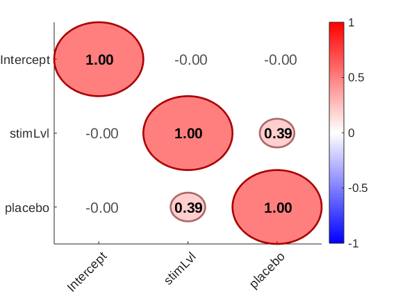
Here is what happens when we use Option 3. This removes the predicted effects of baseline pain from the treatment effect estimates.
We'll use the Empirical Bayes estimates because these are probably the best estimates of individual scores we have.
Note: the resid() function has a flag that preserves the overall mean response so we can remove the covariate without removing the average treatment effects.
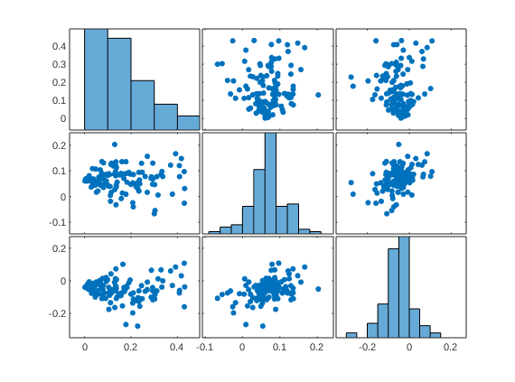
avg_pain = stats.Y_star(:, 1);

% Get new placebo scores
resid_placebo = resid(avg_pain, stats.Y_star(:, 3), true);

resid_stimLvl = resid(avg_pain, stats.Y_star(:, 2), true);

figure; plotmatrix([avg_pain resid_stimLvl resid_placebo]);

plot_correlation_matrix([avg_pain resid_stimLvl resid_placebo], 'names', stats.inputOptions.names);
drawnow, snapnow
2nd-level predictors
Mixed models can include between-person (e.g., group) predictors as well. These could include sex/gender, counterbalancing order variables, and others.
You can include between-person and within-person predictors in any mixed effects model. They can interact with (i.e., moderate) the within-person effects, and/or they can have main effects on the response.
In glmfit_multilevel, these are entered in a second-level design matrix, X2. X2 will automatically include an intercept as the first effect. One block of output stats is included for the average within-person effects (the group intercept), with one block for each of the 2nd-level predictors.
e.g., here, we will include baseline pain as a 2nd-level predictor. The first stats block reports the within-person effects at the average baseline pain, and the second reports baseline pain effects on each within-person effect (the intercept is not of interest here)
Note: you must mean-center all 2nd-level predictors (except the intercept) for the interpretations above to hold. If you do not, your estimates of within-person effects will change and be potentially uninterpretable. Centering will be done automatically UNLESS you explicitly turn it off using the 'nocenter' option.
X2 = cellfun(@nanmean, Y)';

stats = glmfit_multilevel(Y, X, X2, 'names', X_var_names, 'beta_names', {'Average_pain'}, 'weighted', 'boot');
Warning! Some participants have no variance in X column(s) and will be excluded
Participant numbers:80
Analysis description: Second Level of Multilevel Model
GLS analysis

Observations: 120, Predictors:   2
Outcome names: Intercept	stimLvl	placebo
Weighting option: weighted
Inference option: bootstrap

Other Options:
	Plots: No
	Robust: no
	Save: No
	Output file: glmfit_general_output.txt
	R & B - type Empirical Bayes reweighting.
 Min p-value is 0.000000. Needed: 5867 samples
 Bootstrapping 5867 samples... Bootstrap done in 0.02 s, bias correct in 0.00 s
Total time: 0.77 s

________________________________________
Average p-value tolerance (average max alpha): 0.0060

Bootstrapped statistics. Bootstrap inference
	Outcome variables:
	Intercept	stimLvl	placebo
Adj. mean	0.00	1.01	0.01	0.36	-0.01	-0.26

Within-person average effects
	Intercept	stimLvl	placebo
Coeff	0.00	0.01	-0.01
STE	0.00	0.01	0.01
t	0.50	0.68	-1.03
Z	0.82	1.03	-1.24
p	0.40976	0.30380	0.21422


Average_pain
	Intercept	stimLvl	placebo
Coeff	1.01	0.36	-0.26
STE	0.01	0.07	0.09
t	123.11	5.84	-3.58
Z	3.33	3.52	-3.39
p	0.00086	0.00043	0.00070

________________________________________