Create and plot design matrices
Contents
Create and plot your own design matrix easily using CANlab tools! Note: This also requires SPM software functions
These functions are useful for design simulations. They use the following core functions, which may also be useful to use separately if you are doing simulations or building/testing design matrices:
% onsets2fmridesign : Turn a cell array of event onsets into a design matrix, with a chosen basis set
% hpfilter          : High-pass filter a set of data vectors (or design matrix)
% plotDesign        : Make a plot of onsets and regressors
% plot_matrix_cols  : Plot columns of a matrix as lines; useful for visualizing regressors
% create_orthogonal_contrast_set : Create a contrast set that captures space of differences between conditions
% calcEfficiency    : Calculate the efficiency of a set of contrasts (differences).
%                     This is related to power to detect differences across conditions. More is better.
% getvif            : get variance inflation factors for each column (regressor) in a design matrix
%                     These range from 1 (best) to Infinity (worst).
%                     They relate to the ability to accurately estimate the slope for each individual regressor.
%                     They take colinearity (correlation between
%                     predictors) into account, but not variance in the
%                     predictors, which also contributes to efficiency and power to
%                     detect an effect.
%
Note: You need the Matlab stats toolbox on your path. Check for it here:
if isempty(ver('stats')), warning('You do not have the statistics toolbox on your Matlab path. You may/will get errors'); end
Create a simple, one-event design
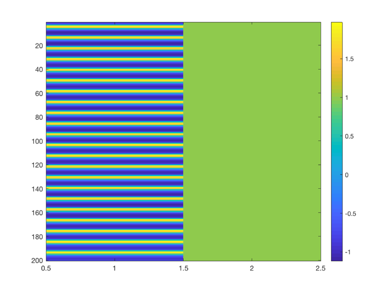
TR = 2;                 % Repetition time for scans; one image every TR; in seconds
ISI = 18;               % Inter-stimulus interval in sec (min time between events)
eventduration = 3;      % Duration of 'neural' events in sec
HPlength = 128;         % High-pass filter length in sec
dononlin = 0;           % Nonlinear saturation model (0 = no, 1 = yes)

create_figure('design');
[X, e] = create_design_single_event(TR, ISI, eventduration, HPlength, dononlin);
drawnow, snapnow

% X is the design matrix.
% Efficiency is e. More is better.
%
% To explore the design matrix, try typing X <and then return> to see the
% values. Remember that the last column is the intercept. The intercept is
% not shown on the plot.  Too see a heatmap of X, you can also try:

figure; imagesc(X); colorbar
drawnow, snapnow
Questions to answer:
% 1. How many columns does X have?
% 2. What does each represent (i.e., a task event type, etc.)?
% 3. Make the events really brief (0.5 sec). What happens to the efficiency?
% 4. Make the events really long (17 sec). What happens to the efficiency?
% 5. Make a plot of the curve showing efficiency from 1 to 18 sec.

% % for dur = 1:18
% %     [X, e(dur)] = create_design_single_event(TR, ISI, dur, HPlength, dononlin);
% % end
% % figure; plot(e)

% When is efficiency maximal?  Why does this make sense?
Create a randomized event-related design with 4 conditions
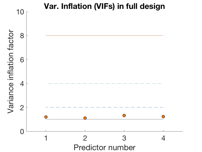
TR = 1;
ISI = 1.3;
eventduration = 1;
freqConditions = [.2 .2 .2 .2];         % Frequencies of each condition, from 0 - 1
HPlength = 128;
dononlin = 0;

create_figure('design');
[X, e, ons] = create_random_er_design(TR, ISI, eventduration, freqConditions, HPlength, dononlin);
axis tight

% Plot the variance inflation factors
create_figure('vifs');
vifs = getvif(X, false, 'plot');

drawnow, snapnow
Variance inflation: 1 (black line) = minimum possible (best)
Successive lines indicate doublings of variance inflation factor.
Red boxes have extremely high VIFs, perfect multicolinearity
Questions to answer:
% 1. How correlated are the regressors? hint: corr.m in Matlab
% 2. What are the VIFs? Are they in an acceptable range?
% 3. Create a new regressor that is a linear combination of the first two.

% Hint:
% % X(:, 4) = .5 * X(:, 1) + .5 * X(:, 2);

% How correlated are they now? Are any regressors perfectly correlated with
% any other one?
% What are the VIFs? As a rule of thumb, VIFs of 1 are ideal, but < 2.5 are reasonable.
% Are these in an acceptable range?
%
% 4. Create a sparse version of the same design, with few events.
%
% % create_figure('design');
% % [X, e, ons] = create_random_er_design(TR, ISI, eventduration, [.05 .05 .05 .05], HPlength, dononlin);
% % axis tight
% % e
%
% Is the efficiency higher or lower?  Why?
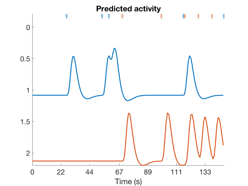
Now create a sparse randomized event design with two event types (conditions) Only 5% of the potential stimulus display time bins are filled with events The rest of the time is rest.
create_figure('design');
[X, e, ons] = create_random_er_design(TR, ISI, eventduration, [.05 .05], HPlength, dononlin);
axis tight

% Create a table object (t) with event onsets and display it
t = table(ons{1}(:, 1), ons{1}(:, 2), ons{2}(:, 1), ons{2}(:, 2), 'VariableNames', {'Evt1_Time' 'Evt1_Dur' 'Evt2_Time' 'Evt2_Dur'});
disp(t);
    Evt1_Time    Evt1_Dur    Evt2_Time    Evt2_Dur
    _________    ________    _________    ________

         26         1           68.9         1
       53.3         1           98.8         1
       58.5         1            117         1
      115.7         1          127.4         1
      146.9         1          137.8         1
Questions to answer:
% 1. Create a dense randomized event design with two conditions, with 100%
% of the time bins filled, spread evenly across 2 event types
%
% % create_figure('design');
% % [X, e, ons] = create_random_er_design(TR, ISI, eventduration, [.5 .5], HPlength, dononlin);
% % v = getvif(X)
%
% The variance inflation factors relate to the estimability of the
% individual regressors. What happens to them as you move from a sparse to
% a dense design?
% The efficiency relates to the ability to detect a contrast effect. Here, this is the difference
% between regression slopes for event 1 vs 2. What happens to the efficiency?
% Why does this make sense?
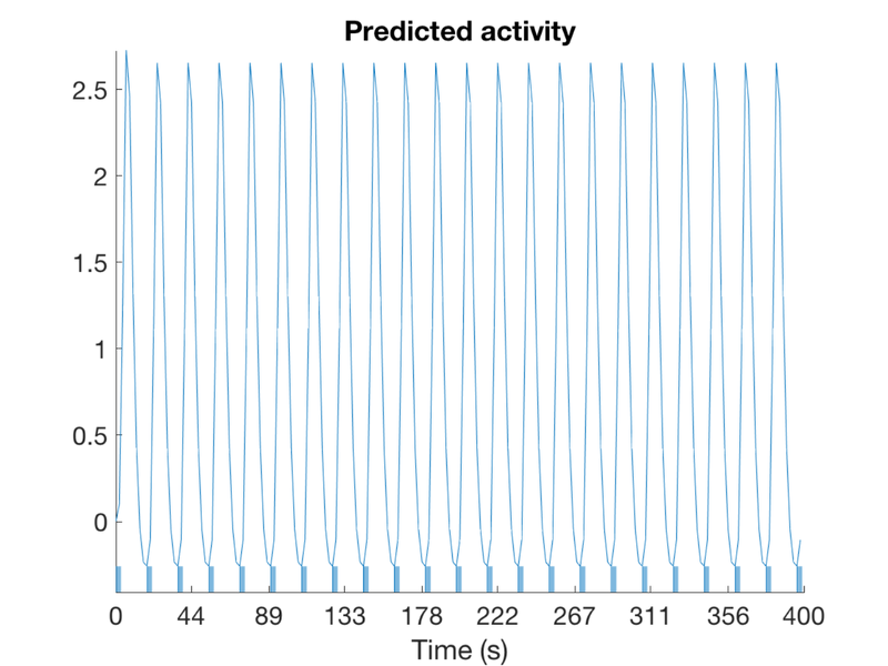
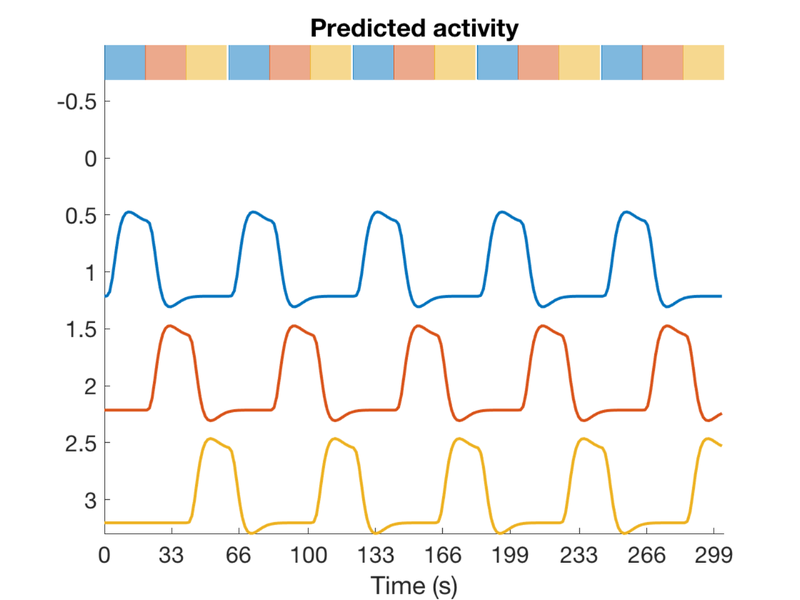
Create an alternating block design with 3 conditions
scanLength = 230 * 1.3;     % 230 frames * 1.3 sec/frame
TR = 1.3;
nconditions = 3;
blockduration = 20;
HPlength = 128;
dononlin = 0;

create_figure('design');
[X, e] = create_block_design(scanLength, TR, nconditions, blockduration, HPlength, dononlin);
axis tight
drawnow, snapnow


% % X(:, 3) = [];
% % v = getvif(X)
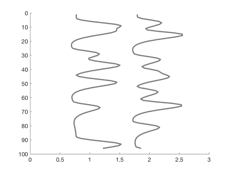
Create a simple design with two event types and pre-specified onsets
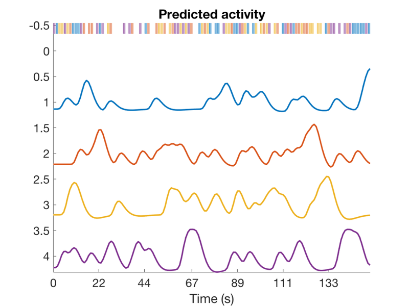
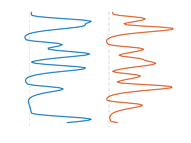
T = 96;  % time points
n = 12;  % number of events

% Create onsets for two events types
events{1} = randperm(T); events{1} = events{1}(1:n)';
events{2} = randperm(T); events{2} = events{2}(1:n)';

% Build model: Convolve with HRF (need SPM on path)
X = onsets2fmridesign(events, 1, T, spm_hrf(1));

% Plot it
create_figure('X');
h = plot_matrix_cols(zscore(X(:, 1:2)), 'vertical');

% Customize
set(h, 'LineWidth', 3);
drawnow, snapnow

% Another plot
create_figure('X 2nd plot');
h = plot_matrix_cols(zscore(X(:, 1:2)), 'vertical');

% Customize
set(h(1), 'LineWidth', 3, 'Color', [0    0.4470    0.7410]);
set(h(2), 'LineWidth', 3, 'Color', [0.8500    0.3250    0.0980]);
hh = plot_vertical_line(1 - .25); set(hh, 'LineStyle', '--');
hh = plot_vertical_line(2 - .25); set(hh, 'LineStyle', '--');
axis tight
axis off
drawnow, snapnow
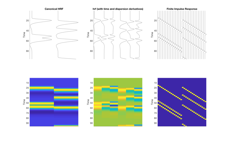
Create a simple design, with three different basis sets
T = 96;  % time points
n = 4;  % number of events

% Create onsets for two event types (conditions)
events{1} = randperm(T); events{1} = events{1}(1:n)';
events{2} = randperm(T); events{2} = events{2}(1:n)';

% Create and display a table of these onset times:

t = table(ons{1}(:, 1), ons{1}(:, 2), ons{2}(:, 1), ons{2}(:, 2), 'VariableNames', {'Evt1_Time' 'Evt1_Dur' 'Evt2_Time' 'Evt2_Dur'});
disp(t)

clear X bfname

% Build three models: Convolve with three basis sets (need SPM on path)
% 1: canonical, 2: 3-parameter, 3: FIR

bfname{1} = 'Canonical HRF';
X{1} = onsets2fmridesign(events, 1, T, spm_hrf(1));

bfname{2} = 'hrf (with time and dispersion derivatives)';
X{2} = onsets2fmridesign(events, 1, T, bfname{2});

bfname{3} = 'Finite Impulse Response';
X{3} = onsets2fmridesign(events, 1, T, bfname{3});

create_figure('X_3basis sets', 2, 3);

for i = 1:3

    subplot(2, 3, i)
    h = plot_matrix_cols(zscore(X{i}(:, 1:end-1)), 'vertical');
    set(gca, 'XColor', 'w', 'YTick', [0:20:100]);
    axis tight
    title(bfname{i})
    ylabel('Time')

    subplot(2, 3, 3+i)
    imagesc(X{i}(:, 1:end-1))
    set(gca, 'YDir', 'Reverse', 'XTickLabel', []);
    ylabel('Time')
    axis tight

end

drawnow, snapnow
    Evt1_Time    Evt1_Dur    Evt2_Time    Evt2_Dur
    _________    ________    _________    ________

         26         1           68.9         1
       53.3         1           98.8         1
       58.5         1            117         1
      115.7         1          127.4         1
      146.9         1          137.8         1
Questions to answer:
% 1. What is the interpretation of each of the columns? Which event type
% and which effect is represented?
%
% 2. Would it make sense to calculate contrasts across regressors 1 and 2
% of design matrix #1?
% How about design matrix #2?
%
% 3. What contrast weights would capture the difference in the canonical
% HRF regressor amplitudes between event type 1 and 2, for Model 1?  For
% Model 2?
Simulate data and model fits
We'll create simulated data that responds to only one event type with a typical canonical response (+ noise)
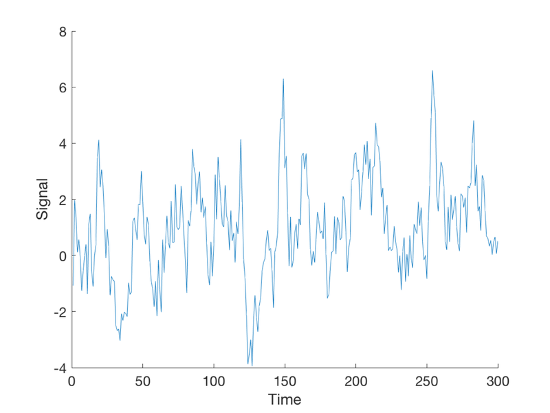
Create a longer design with more events:
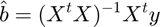
T = 300;    % time points
n = 20;     % number of events per condition
TR = 1;     % Time per image (sec)
ISI = 2;
eventduration = 1;

% Create onsets for two event types
events{1} = randperm(T); events{1} = events{1}(1:n)';
events{2} = randperm(T); events{2} = events{2}(1:n)';

% To visualize this:
% % plotDesign(events, [], TR);
% % drawnow, snapnow


% Now we need to simulate data using known, true parameters
% X gives us plausible curves for true responses

X = onsets2fmridesign(events, 1, T, spm_hrf(TR));

% Standarize the regressors to have a standard deviation of 1
% This makes it convenient to add a noise signal with the same standard
% deviation later, so we can control the signal to noise ratio:
X(:, 1:2) = X(:, 1:2) ./ std(X(:, 1:2));

% We'll use y for simulated data.
% The true response is an amplitude=1 response to event type #1 alone

b_true = [1 0 0]';                     % these are the *true* regression slopes
y_true = X * b_true;

% Create some autocorrelated noise:
e = noise_arp(T, [.5 .2]);

% The observed response is the true signal + error:
y = y_true + e;

create_figure('observed data (y)');
plot(y)
xlabel('Time')
ylabel('Signal')
To fit the model, we calculate the projection of the data onto the model space. The betas (b vector) are the regression slopes. In linear algebraic terms, the model is:
And the solution is this:
In code:
b = inv(X' * X) * X' * y;
The fitted response is as close as we can get in the model space, and equals the predictors multiplied with the betas:
$$ \hat{y} = X\hat{\beta};
The fitted response is as close as we can get in the model space, and equals the predictors multiplied with the betas:

In code:
fit = X * b;
Plot the fitted response
plot(fit)
legend({'Data' 'Fit'});
drawnow, snapnow
Now we'll make a table with the true and estimated betas side by side
t = table(b_true, b, 'VariableNames', {'True' 'Estimated'});
disp(t)
    True    Estimated
    ____    _________

     1         1.0333
     0      -0.049884
     0        0.26248
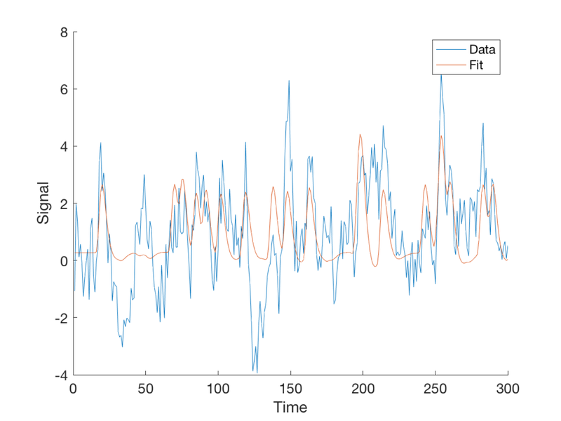
Explore the FIR model fit
X_fir = onsets2fmridesign(events, 1, T, 'Finite Impulse Response');

b = inv(X_fir' * X_fir) * X_fir' * y;

% Now get the betas for each event type
% These represent the estimated activity at each time following event onset
% Together, these are the estimated HRF shape
% (The last column is the intercept. We'll ignore it in our plots.)
% The first k betas are for Event Type 1:

k = (length(b) - 1) / 2

t = 1:2:30; % t is time since stimulus. b's are in units of 1 per 2 sec by default

create_figure('Estimated HRF')
plot(t, b(1:k), 'LineWidth', 3);     % Event 1
plot(t, b(k+1:2*k), 'LineWidth', 3); % Event 2
legend({'Event 1' 'Event 2'})
xlabel('Time since stimulus')
ylabel('Response')
k =

    15


ans =

  Figure (Estimated HRF) with properties:

      Number: 8
        Name: 'Estimated HRF'
       Color: [1 1 1]
    Position: [680 558 560 420]
       Units: 'pixels'

  Use GET to show all properties
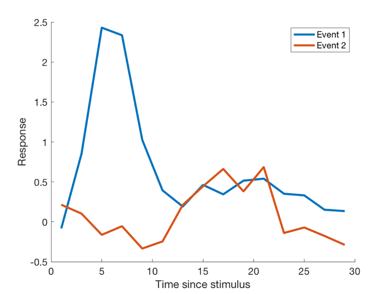
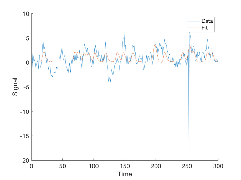
Now let's add an outlier time point.
when = min(T, floor(events{1}(1) + 6));
y(when) = -20;

create_figure('observed data (y)');
plot(y)
xlabel('Time')
ylabel('Signal')

% Fit the model
b = inv(X' * X) * X' * y;

disp('With an outlier:')
t = table(b_true, b, 'VariableNames', {'True' 'Estimated'});
disp(t)
With an outlier:
    True    Estimated
    ____    _________

     1       0.80265
     0      0.012366
     0       0.30015
Plot the fitted response
fit = X * b;
plot(fit)
legend({'Data' 'Fit'});

% save the figure handle so we can re-activate it and add to it:
fighan = gcf;
Another way to look at this is with a scatterplot Notice the outlier!
create_figure('scatter');
scatter(fit, y, 'MarkerFaceColor', [.3 .2 .6]);
xlabel('Fitted response (based on X)');
ylabel('Observed response (brain)');
h = refline;
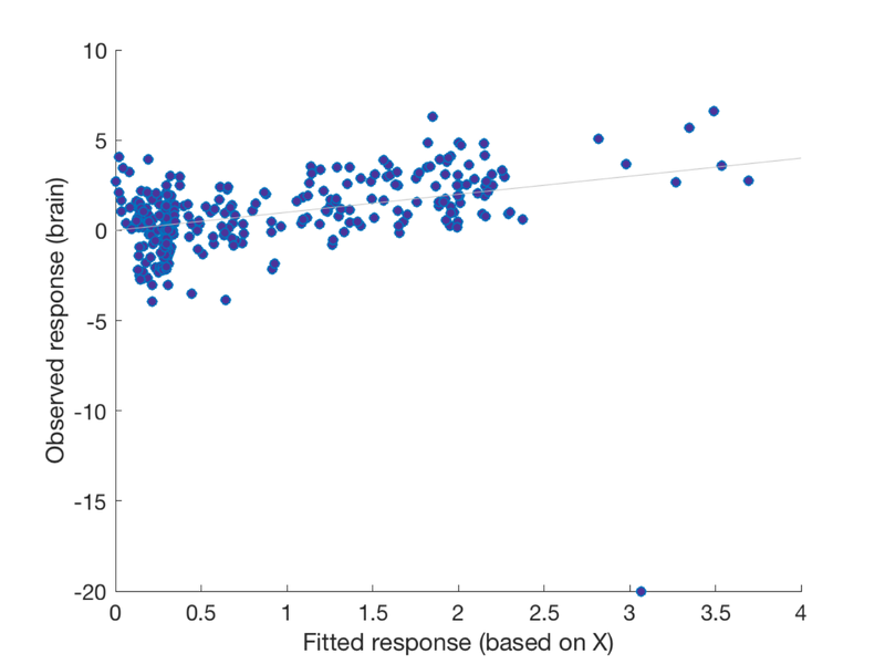
Questions to answer:
% 1. If the outlier were farther out on the x-axis (predictor axis), i.e.,
% more extreme, would you expect it to have more or less pull on the
% regression line?
%
Now let's make a new outlier at an extreme X value.
wh = find(X(:, 1) == max(X(:, 1)));
y(wh) = -10;

% 2. Re-plot the scatterplot and show the new graph
% 3, Re-activate the fit figure and add the new fit

% % figure(fighan)          % re-activate the old figure
% % plot(fit)
% % legend({'Data' 'Fit' 'Robust Fit'});
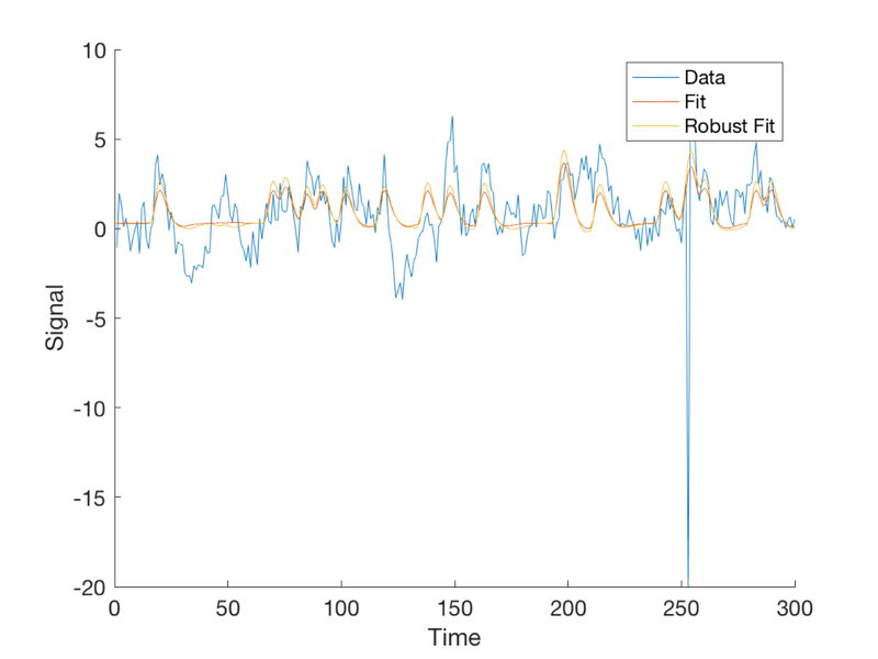
Now we'll try the fit with robust regression instead Robust regression with robfit adds an intercept to the first column of the design matrix automatically, so we'll remove the intercept when we pass it in, then rearrange the betas so that the intercept is last again, to match our other models.
[b_rob, stats] = robustfit(X(:, 1:2), y);

b_rob = [b_rob(2:end); b_rob(1)];
Get and plot the fit
rob_fit = X * b_rob;

figure(fighan)          % re-activate the old figure
plot(rob_fit)
legend({'Data' 'Fit' 'Robust Fit'});

% *Questions to answer:*

% 1. When does the robust regression make the most difference? Why?