Feature map
A visual map of all 103 annotation channels and their hierarchical organization — the six feature classes, each grouped by subclass, with one chip per channel.
Editable graphic
The map is a plain, flat SVG built for editing:
analysis/figures/feature_map.svg.
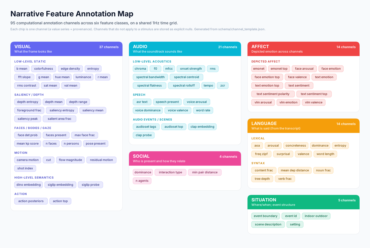
- Open it in PowerPoint, Illustrator, Inkscape, or any browser. In PowerPoint, Insert → Pictures, then right-click → Convert to Shape to recolor, move, or relabel individual cards, chips, and text.
- It uses real text elements, per-card groups, and inline colors (no CSS or filters), so it survives import cleanly and recolors easily.
- Regenerate it whenever the channel set changes:
python3 tools/build_feature_map.py # reads schema/channel_template.json
Feature summary table
Feature groups organized by class (row) and by level of abstraction (column). Numbers in parentheses are the count of variables in that group — each scalar/flag counts as 1 and each vector counts as its dimensionality (so an embedding contributes many). “Level” is the standard perception hierarchy: low-level = raw physical/perceptual signal, mid-level = perceptual organization/structure, high-level = semantic/conceptual.
| Feature class | Low-level | Mid-level | High-level |
|---|---|---|---|
| Visual | image statistics (12); optical-flow motion (3); shot cuts (2) | saliency & depth (8); faces & bodies (7) | SigLIP semantics — embedding + scene probes (784); DINOv2 embedding (384); action recognition (400) |
| Audio | acoustics — loudness / pitch / timbre / MFCC / chroma (34) | speech presence & rate (2) | AudioSet sound tags (527); CLAP semantics — embedding + probes (524); vocal affect V/A/D (3) |
| Language | word frequency & length (2) | lexical norms — valence / arousal / dominance, concreteness, AoA (5); syntactic complexity (5) | word surprisal & entropy (2); LLM embeddings — Qwen3 (1024) + Llama-3.1 AR (4096); semantic coherence/drift/novelty/surprise (4); narrative expectedness/surprise (2) |
| Social | — | agent count & closest-pair distance (2) | interaction type & social dominance (2) |
| Situation | — | — | scene description / setting / indoor–outdoor (3); event structure — boundaries & event id (2) |
| Affect | — | facial affect — 8 expressions + valence + arousal (10) | EmoNet image emotion (20); text emotion & sentiment (32); VLM depicted emotion (3) |
A one-page Word version of this table (for import into Google Docs) is at
docs/feature_summary_table.docx, regenerated bypython3 tools/build_feature_summary.py.
The major feature types
What each model in the pipeline is, what it outputs, why it is useful (with an eye to
fMRI encoding / brain–feature modeling), and the canonical reference. Counts in
parentheses match the chips above. Reference links go to the public paper; local PDF
copies live in PDFs/ (Dropbox-only).
Visual — what the frame looks like
-
Low-level image statistics (12) — Classic per-frame pixel/color measures computed with scikit-image: luminance, RMS contrast, mean red/ green/blue and hue/saturation/brightness, edge density, image entropy, the slope of the spatial-frequency (Fourier) power spectrum, and perceptual colorfulness (Hasler & Süsstrunk 2003). These are the cheapest, most reproducible visual regressors and the standard low-level controls in vision/fMRI work — early visual cortex (V1–V2) tracks luminance, contrast, and spatial-frequency energy closely, so they are essential nuisance/target regressors before attributing signal to higher-level features.
-
SigLIP 2 embedding (768) + scene probes (16) — Google’s SigLIP 2 is a contrastive vision–language model (a Vision Transformer trained to align images with text). It converts each frame into a 768-dimensional semantic embedding, and by scoring the frame against short text prompts it also yields 16 interpretable scene-probe values (e.g. indoor/outdoor, nature, faces, text). The embedding is a strong general-purpose semantic space for encoding/RSA models of higher visual and category-selective cortex; the probes give human-readable scene descriptors.
-
DINOv2 embedding (384) — Meta AI’s DINOv2 is a self-supervised Vision Transformer that turns an image into general-purpose visual features without using any labels or text. Its 384-d global embedding captures objects, parts, texture, and layout, and is a leading backbone for representational- similarity analysis, linear-probe decoding, and voxelwise encoding of ventral-stream responses — complementary to SigLIP because it is label-free (vision-only).
-
Action recognition (400) — VideoMAE (masked- autoencoder video Transformer, fine-tuned on Kinetics-400) reads a short clip and outputs a probability over 400 human-action categories (e.g. running, dancing, cooking, shaking hands, playing guitar). The pipeline stores the full 400-value probability vector plus the single top action label per second — a semantic “what are people doing” regressor for action-observation and social/motor brain systems.
-
Motion — optical flow (3) — RAFT estimates dense per-pixel motion between consecutive frames. From it the pipeline derives overall optical-flow magnitude, a camera-motion estimate, and residual (object) motion. Low- level motion energy is a classic driver of MT/MST and dorsal-stream responses and a standard motion regressor in naturalistic fMRI.
-
Shot cuts & shot index (2) — A histogram-based cut detector (a lightweight stand-in for TransNetV2) flags edit boundaries and numbers the shots. Cuts are strong low-level visual-transient events and useful for modeling attention/event-onset responses.
-
Faces & bodies (7) — MTCNN detects faces (count, detection confidence, largest-face size, face-present flag) and Keypoint R-CNN (from the Mask R-CNN family) detects human body pose (person count, pose confidence, body-present flag). Face presence/size is a primary regressor for face-selective cortex (FFA/OFA/STS); body/person presence drives EBA and the person-perception network.
-
Saliency & depth (8) — A spectral-residual saliency model (Hou & Zhang 2007; stand-in for a deep video-saliency net) gives where the eye is likely drawn (mean/peak saliency, spread, salient-area fraction), and Depth-Anything-V2 gives monocular depth (mean depth, depth range, depth complexity, foreground fraction). Saliency proxies bottom-up attention; depth/near-far structure relates to scene-geometry coding (PPA/OPA).
Audio — what the soundtrack sounds like
-
Low-level acoustics (34) — librosa computes loudness (RMS), spectral shape (centroid, bandwidth, rolloff, flatness), zero-crossing rate, onset strength, a 13-value MFCC timbre vector, and a 12-value chroma (musical pitch-class) vector; pitch/F0 uses pYIN and tempo uses dynamic-programming beat tracking (Ellis 2007). These are the standard acoustic regressors for auditory-cortex encoding (loudness/spectral envelope track Heschl’s-gyrus responses).
-
AudioSet sound tags (527) — the Audio Spectrogram Transformer (AST) classifies each ~1 s window into 527 sound-event categories from Google’s AudioSet ontology (speech, music, laughter, vehicles, animals, gunshots, applause, weather, …). The pipeline stores the full 527-value tag vector plus the top tag — a rich semantic description of the auditory scene for modeling category-selective auditory and associative regions.
-
CLAP audio embedding (512) + sound probes (12) — CLAP is a contrastive language–audio model (the audio analogue of CLIP): it embeds each audio window into a 512-d space aligned with text, so arbitrary text prompts (“a crowd cheering”, “tense music”) can be scored against it. The pipeline keeps the 512-d embedding and 12 interpretable sound probes. The embedding is a general auditory-semantic feature space for encoding models.
-
Speech (5) — faster-whisper (Whisper) transcribes speech and yields a speech-present flag and speaking rate (words/s); audEERING wav2vec2 reads vocal affect directly from the voice as continuous valence, arousal, and dominance. Speech presence and speaking rate are core language-network regressors; vocal affect targets prosody/emotion circuits (e.g. voice-sensitive STS, amygdala).
Language — what is said (from the transcript)
-
Lexical semantic norms (5) — per word, human-rated norms are looked up: emotional valence, arousal, dominance (Warriner 2013), concreteness (Brysbaert 2014), and age of acquisition (Kuperman 2012). These are the classic word-property regressors for language and semantic fMRI.
-
Word frequency & length (2) — wordfreq gives each word’s log frequency (Zipf scale) and its length. Frequency is a robust predictor of lexical-access difficulty and reading/listening time.
-
Surprisal & next-word entropy (2) — GPT-2 provides each word’s surprisal (how unexpected it was, in bits) and the entropy of the model’s next-word prediction. Word-by-word surprisal from language models is one of the most reliable predictors of language-network and N400-type responses in naturalistic-comprehension fMRI/MEG.
-
Syntax (5) — spaCy parses each utterance for content-word fraction, noun/verb fraction, parse-tree depth, and mean dependency distance — proxies for syntactic complexity and processing load.
-
LLM language embeddings (5120) — a dense, contextual representation of what is said, mirroring SigLIP/CLAP for the other modalities. Qwen3-Embedding (Alibaba, 2025) gives a 1024-d sentence embedding per utterance, and Llama-3.1-8B supplies 4096-d autoregressive hidden states — the standard feature for fMRI/MEG language-encoding models. Aligned to whisper word timings and resampled to 1 Hz.
-
Semantic & narrative surprise (6) — interpretable scalars derived from the embeddings at rising levels: semantic coherence / drift / novelty / surprise (how the meaning of each line relates to what came before, from the Qwen3 embeddings) and narrative expectedness / surprise (how predictable each line is given the story so far, rated by Llama-3.1-8B-Instruct). Together with GPT-2 word surprisal and spaCy syntax, these span lexical → semantic → discourse/narrative prediction error.
Social — who is present and how they relate
- Social relations (4) — derived from the video by the Qwen2.5-VL vision-language model (interaction type, social dominance) plus face/pose detectors (MTCNN agent count; Keypoint R-CNN closest-pair distance). These target the social-perception network (STS, TPJ, mentalizing regions) that tracks the number of agents, their proximity, and the type of interaction.
Situation — where/when; event structure
- Scene & setting (3) — the Qwen2.5-VL VLM produces a free-text scene description, an indoor/outdoor label, and a coarse setting label per second — high-level context for scene/place-selective cortex.
- Event boundaries (2) — GSBS (Greedy State Boundary Search; Geerligs 2021) segments the annotation time series into discrete “events,” emitting boundary events and a running event number. This directly operationalizes event-segmentation theory and models the boundary responses seen in hippocampus and default-mode regions during naturalistic viewing.
Affect — depicted emotion across channels
Emotion is read from several independent channels/modalities so it can be cross-validated (facial, textual, and holistic-scene here; vocal affect lives under Audio → Speech):
-
EmoNet — image emotion (20) — EmoNet (Kragel et al. 2019, Science Advances) is an AlexNet-based CNN that maps a video frame onto 20 emotion categories (e.g. amusement, awe, fear, sexual desire, horror, joy, sadness). It was trained to predict the emotion evoked by images and validated against human ratings and brain responses, making it a purpose-built regressor for visual emotion-category coding in the brain.
-
Facial affect (10: 8 expressions + valence + arousal) — HSEmotion (Savchenko) reads faces detected in the video and classifies expression into 8 categories (anger, contempt, disgust, fear, happiness, neutral, sadness, surprise) plus continuous facial valence and arousal — targeting emotion read-out from faces (amygdala, STS, face network).
-
Text emotion & sentiment (28 + 3) — from the transcript, GoEmotions RoBERTa scores 28 fine-grained emotions (admiration, gratitude, grief, …) and CardiffNLP RoBERTa scores 3-way sentiment (negative/neutral/positive) with a continuous polarity. These capture the emotional content of what is said.
-
VLM depicted emotion (3) — Qwen2.5-VL also judges the overall depicted emotion, valence, and arousal of the scene as a holistic cross-check on the specialized channels.
Related
- The designed semantic hierarchy behind these channels (the taxonomy the pipeline is organized around): feature hierarchy.
- What each pass actually computes: pipeline status.
- The full per-model survey (all surveyed tools, with references): the scoping review sections.
- The on-disk layout of these channels in each
.h5: annotation format.