CANlab Second-level analysis batch system
The batch system, specialized for second-level neuroimaging data analysis, is in CANlab_help_examples repository.
See batch workflow for a walkthough of the batch scripts. The walkthrough is also presented below.
| Sections on this page |
|---|
| Philosophy |
| WHAT THESE TEMPLATE SCRIPTS ARE AND WHAT THEY DO |
| DEPENDENCIES |
| FEATURES |
| QUICK START: SETTING UP A NEW ANALYSIS FOR A NEW DATASET |
| RUNNING ANALYSES AND GENERATING REPORTS |
| OVERVIEW OF SCRIPTS IN THE FOLDER AND WORKFLOW |
| Step 1: Create a folder and run the setup script |
| Step 2: Edit files in you local analysis folder and save |
| Step 3: Load and prepare contrast images and analyses |
| Step 4: Run scripts to generate on-demand results |
| Step 5: Run batch scripts to publish date-stamped HTML reports |
| MORE INFO ABOUT HOW FILES AND VARIABLES ARE STORED |
Batch scripts: Philosophy
This page describes a system of batch scripts located in the CANlab_help_examples repository, in the Second_level_analysis_template_scripts folder. The batch system is designed to facilitate second-level analysis across a series of activation estimate or contrast images from a group of participants. This provides a lightweight dataset with a set of standard analyses that can be used in publication, shared, and archived. The scripts are designed with the following values in mind:
Transparency: Scripts are simple to read, write, and interpret, re-using the same variable names. This increases readability and reduces coding errors.
Efficiency: A batch system built on simple object commands runs a variety of standard quality control checks and analyses. “Prep_” scripts are run once and do most of the heavy lifting, saving files with standard file and variable names. These can be loaded and re-run on-demand to generate results reports.
Reproducibility: The scripts are designed to be easily re-run to reproduce all the analyses, figures, and statistics, including HTML reports.
Minimization of errors: Scripts that do standard analyses are re-used and vetted across analyses and users, reducing coding errors.
Provenance and history “Publish” scripts save date-stamped HTML reports with figures and statistics. This provides a base set of analyses that reduces coding time and reduces coding errors. This is good for archiving and reproducibility, and good for efficiently writing papers.
Shareability: Standardized variable names make it easy to understand the structure of the folders and files, which promotes meaningful sharing. Date-stamped HTML reports provide a record of analyses, figures and statistics that can be archived and shared.
Flexibility: The batch scripts provide a series of modules that can be “mixed and matched”, and customized, depending on the needs for a particular study.
Extensibility: The batch scripts are extensible, and serve as a kind of template to create and “plug in” new analyses.
Other walkthroughs
Interactive analysis walkthroughs: Another series of help files is a series of step-by-step analysis walkthroughs are in the CANlab_help_examples repository, in the example_help_files folder.
Simple (alternative) batch system: Also, there is a very simple set of batch scripts suitable for other analytic purposes in the CANlab_help_examples repository, in the Canlab_simple_image_load_prep folder. This uses the same philosophy of defining a clear path to re-load saved files with standardized variable names, but is simpler and much more bare-bones than the full batch system. It can be useful when prototyping new analyses that do not fit into the batch system.
CANlab second-level batch scripts
https://www.github.com/Canlab https://github.com/canlab/CANlab_help_examples
WHAT THESE TEMPLATE SCRIPTS ARE AND WHAT THEY DO
This is a set of scripts that is designed to facilitate second-level analysis across beta (COPE), or contrast images from a group of participants. It’s particularly helpful for signature-based analysis of group data, usually starting with beta images (one image per subject per condition) produced by first-level GLM analyses. It assumes that you are starting with Analyze (.img) or NIFTI (.nii) files from a first-level analysis, and that these images are in MNI space.
Think of it as a framework that standardizes variable names and file formats, and makes it easy to run analyses and save HTML reports without writing a bunch of custom code.
There are four kinds of files in the batch system. prep_[1 2 3 etc.] scripts set up data structures and files and need only be run during initial setup (once) Scripts named a_ b_ c_ etc. run analyses and print reports using the prepped files.
*z_batch** scripts run sets of other scripts. Those with “publish” in the filename generate HTML reports. *plugin_** scripts are for internal use and keep the code clean. You should not need to edit these or run them directly.
The philosophy is to have scripts with standardized variable names and minimal editing required to adapt them to a new dataset.
Also, these scripts include ‘batch’ scripts that run analyses and save HTML files with results and images, storing a time-stamped record of your analysis.
In principle, you should only need to edit two scripts to customize the analysis for a new dataset:
a_set_up_paths_always_run_first.m prep_1_set_conditions_contrasts_colors.m
Then the rest should run correctly, for most datasets.
The master scripts to edit are in the folder Second_level_analysis_template_scripts. You do not have to copy over all the scripts from the master scripts folder to use them. You can run the master scripts directly from the master copy.
- the standard versions of most of the master scripts will run without editing.
- If you want to customize a script or create new scripts, do not edit the master scripts. Instead, can copy any of them to your local project scripts folder and customize them. Those customized versions will be run instead of the standard versions.
DEPENDENCIES
The scripts require several other toolboxes: See https://github.com/canlab/CANlab_help_examples/blob/master/README.md
FEATURES
- Time-stamped HTML printouts of all figures and results for archival/reference purposes
- Short, modular scripts are easy to customize and extend
- Common naming and data storage conventions across all analyses increase readability and organization
- Separate process for loading/preparing datasets/contrasts and running analyses, to make it easier to re-run analyses quickly
- Loading and visualization of all image sets in fmri_data for quality checks
- Extraction of global gray, white, and CSF components
- Quality plots and warning messages based on CSF components’ relationship with gray matter and other measures
- Regression-based rescaling of data to remove CSF components
- Easily customizable specification of contrasts and colors
- Voxel-wise maps for each contrast
- SVM classifier maps for each contrast
- Between-person contrasts and between-condition contrasts if different conditions include different subjects
- Extraction of the NPS and subregions
- Plots and stats on NPS responses by condition and for each contrast
- Extraction, plots, and stats on other signatures (these require access to the private CANlab masks repository): Vicarious pain (VPS), Negative emotion (PINES), Rejection, autonomic signatures, fibromyalgia, cerebral contributions to pain (SIIPS1)
- Extraction, plots, and stats on Buckner Lab resting-state component maps
- Polar plots and ‘river plots’ for relationships between image sets/contrasts and resting-state maps/signatures
- You can load and integrate text summaries and interpretation into your HTML report file.
QUICK START: SETTING UP A NEW ANALYSIS FOR A NEW DATASET
This section describes how to set up and prep an analysis, in 12 steps.
First, make sure you have the CANlab_help_examples and CANLab_Core_Tools repositories on your matlab path:
- Download the CANlab Core Tools repository for neuroimaging data analysis https://github.com/canlab/CanlabCore
- Open Matlab and change to the directory where you want to install the toolboxes (i.e., drag folder into Matlab cmd window)
- Run
canlab_toolbox_setup.m(in Canlab_Core) by dragging the file from Finder/Explorer into Matlab
Once you have the tools installed, you are ready to set up a new analysis.
- Make sure you have a master study analysis folder, MASTER_FOLDER_NAME
- Make a ‘data’ subdirectory
- Add MNI-space .nii/.img+.hdr files to be analyzed there.
- Change to MASTER_FOLDER_NAME in Matlab
- Type
a_set_up_new_analysis_folder_and_scriptsto make subfolders and copy in key files Edit your local copies of
a_set_up_paths_always_run_first.mandprep_1_set_conditions_contrasts_colors.m- Now that the analysis is set up, you’ll run a “prep” script sequence to load data into fmri_data objects, create and run contrasts, and prep Matlab .mat data files. You only need to run this once:
a_set_up_paths_always_run_first.m prep_1_set_conditions_contrasts_colors.m prep_2_load_image_data_and_save.m prep_3_calc_univariate_contrast_maps_and_save.m prep_4_apply_signatures_and_save
This saves files that are re-loaded later and used in analyses. Other “prep_*” scripts can be run, too, including a script that loads behavioral data.
After you have run these, you are ready to reload your saved files and generate results, tables, and HTML reports.
- Once you have your “prep_” running right with no errors, run the batch script
z_batch_publish_image_prep_and_qc
This runs the data-prep process and saves a date-stamped record, with plots, in ‘MASTER_FOLDER_NAME/results/published_output’
- For more help, see the help documents/walkthrough in the canlab_help_examples repository. They are called:
0_CANLab-Help2ndlevelExampleWalkthrough.pdf 0_begin_here_readme.m 0_debugging_common_errors.rtf
See: https://github.com/canlab/CANlab_help_examples/blob/master/README.md
RUNNING ANALYSES AND GENERATING REPORTS
- First, always run
a_set_up_paths_always_run_first.m, so that your paths and folder names will be set. - Then, run
b_reload_saved_matfiles.m, which will load the data files. After that, you can run any of the analysis scripts below.
- You can also run
z_batch_publish_analyses.m, which runs a whole list of analysis scripts and saves the results in an html file (as well as individual figures) in the ‘results’ subfolder.
OVERVIEW OF SCRIPTS IN THE FOLDER AND WORKFLOW
This section contains a more detailed overview of the workflow, and the various scripts you will run to prep the analysis and generate results.
Step 1: Create a main analysis folder MASTER_FOLDER_NAME and navigate there
Run:
| Script | Function |
|---|---|
a_set_up_new_analysis_folder_and_scripts | Creates local folders and copies in relevant scripts |
Step 2: Edit these files in you local analysis folder and save:
| Script | Function |
|---|---|
study_info.json | File with study/author meta-data, for reports and archive |
a_set_up_paths_always_run_first.m | Modify to specify your local analysis folder name |
a2_set_default_options.m | Options used in various other scripts; change if desired, or not |
prep_1b_prep_behavioral_data.m / prep_1b_example2.m | Optional: Modify one of these to load and attach behavioral data from files, e.g., from Excel |
prep_1_set_conditions_contrasts_colors.m | Modify: Specify image file subdirs, wildcards to locate images, condition names and contrasts across conditions |
prep_1c_normalize_to_MNI.m | Optional script to modify and use only if data are not yet in MNI space; otherwise ignore |
prep_0_batch_run_once.m | Batch script to run a whole sequence of prep_* files. |
Step 3: Load and prepare contrast images and analyses:
You only need to run this once if it runs correctly. Relevant info is extracted from images and saved in standard variable names for reloading and results-on-demand later.
| Script | Function |
|---|---|
| a_set_up_paths_always_run_first.m | Always run this first before you run other scripts. Runs: a2_set_default_options |
| prep_1b_prep_behavioral_data.m / prep_1b_example2.m | Optional: Run these load and attach behavioral data from files, e.g., from Excel |
| prep_1_set_conditions_contrasts_colors.m | Modify to specify image file subdirectories, wildcards to locate images, condition names |
| prep_2_load_image_data_and_save.m | Load image data into fmri_data objects and save |
| prep_3_calc_univariate_contrast_maps_and_save.m | Apply contrasts to fmri_data objects |
| prep_3a_run_second_level_regression_and_save.m | [Optional] if you have entered continuous regressors in prep_1b, run regression |
| prep_3b_run_SVMs_on_contrasts_and_save.m | [Optional] run cross-val SVMs on within-person contrasts |
| prep_3c_run_SVMs_on_contrasts_masked.m | [Optional] run cross-val SVMs on within-person contrasts, within a mask |
| prep_3d_run_SVM_betweenperson_contrasts.m | [Optional] run cross-val SVMs across conditions, assuming subjects nested within conditions (e.g., if diff conditions are diff subjects) |
| prep_4_apply_signatures_and_save.m | Apply CANlab signature patterns and attach output (values) to saved DAT structure |
| prep_5_apply_shen_parcellation_and_save.m | [Optional] Extract data from each condition or contrast averaged over each parcel, save file with values |
| prep_5b_apply_spmanatomy_parcellation_and_save.m | [Optional] Extract data from each condition/contrast averaged over each parcel, save file with values |
| prep_6_apply_kragel_emotion_signatures_and_save.m | [Optional] Apply Kragel emotion signature patterns and attach output (values) to DAT |
An alternative, once you feel comfortable with the setup, is to run a batch script with this sequence. All scripts with ‘publish’ in the name print date-stamped HTML reports.
z_batch_publish_image_prep_and_qc.m
Step 4: Run scripts to generate on-demand results:
Always ‘set up paths’ and ‘reload’ before you do anything else. After that, these scripts should (theoretically) be runnable in any order to generate figures and tables of results. The scripts use simple commands and are designed to be guides for you to add your own custom scripts if you want to, and to pick and choose for your study.
Think of them as a menu of items that you may want to run. Batch scripts (below) run collections of these scripts and group them into published HTML reports.
| Script | Function |
|---|---|
| a_set_up_paths_always_run_first.m | Always run this first before you run other scripts. |
| b_reload_saved_matfiles.m | Run this to reload saved and prepped files [Do not modify] |
| b1_behavioral_analysis.m | Optional: Modify/customize for your study. The default script is an example only. |
For all the scripts below, you can run them ‘out of the box’ without customizing them for your study, as long as your prep_* scripts have run correctly and you have reloaded data with a_set_up_paths_always_run_first + b_reload_saved_matfiles
| Script | Function |
|---|---|
| b2_show_data_vs_underlay.m | Show first condition image over canonical brain to check registration and coverage. |
| Contrasts: | |
| c_univariate_contrast_maps.m | Show voxel-wise maps for all contrasts, FDR-corrected and uncorrected; tables |
| c3_univariate_contrast_maps_scaleddata.m | Show voxel-wise contrast maps for scaled/cleaned data |
| c4_univ_contrast_wedge_plot_and_lateralization_test.m | Test contrasts and lateralization across 16 large-scale rsFMRI networks with L/R divisions |
| c5_univ_contrast_wedge_plot_and_lateralization_test_scaled_data.m | Test contrasts and lateralization with scaled data |
| Support Vector Machines: | |
| c2_SVM_contrasts.m | Show SVM results (from prep_3b_run_SVMs_on_contrasts_and_save) |
| c2_SVM_contrasts_masked.m | Show SVM results (from prep_3b_run_SVMs_on_contrasts_masked) |
| c2b_SVM_betweenperson_contrasts.m | Show SVM results (from prep_3d_run_SVM_betweenperson_contrasts) |
| c2c_SVM_between_condition_contrasts.m | Show SVM results (run-on-demand, no prep script yet) |
| Multivariate regression: | |
| c2a_second_level_regression.m | Show regression results (from prep_3a_run_second_level_regression_and_save) |
| c2d_lassoPCR_contrasts.m | Multivariate cross-validated regression results (for, e.g., linear contrasts across multiple conditions) |
| Pre-defined signatures: | |
| d1_pain_signature_responses_dotproduct.m | Test and report extracted ‘signature’ responses (from prep_4_apply_signatures_and_save) |
| d2_pain_signature_responses.m | Test and report extracted ‘signature’ responses with cosine_similarity metric (from prep_4_apply_signatures_and_save) |
| d3_plot_nps_subregions.m | Test and report Neurologic Pain Signature subregions (from prep_4_apply_signatures_and_save) |
| d3_plot_nps_subregions_bars.m | |
| d4_compare_NPS_SIIPS_scaling_similarity_metrics.m | Test and report extracted ‘signature’ responses with multiple similarity metrics (from prep_4_apply_signatures_and_save) |
| d5_emotion_signature_responses.m | |
| d6_empathy_signature_responses.m | |
| d7_autonomic_signature_responses.m | |
| d8_fibromyalgia_signature_responses.m | |
| d9_nps_correlations_with_global_signal.m | Test and report NPS correlations with extracted global gray/white/CSF averages |
| d10_signature_riverplots.m | ‘River plots’ show relationships between each condition (and contrast) and a set of ‘signatures’ |
| d11_signature_similarity_barplots.m | Bar plots showing relationships between each condition (and contrast) and a set of ‘signatures’ |
| d12_kragel_emotion_signature_responses.m | |
| d13_kragel_emotion_riverplots.m | |
| d14_kragel_emotion_signature_similarity_barplots.m | |
| Pre-defined networks: | |
| f2_bucknerlab_network_barplots.m | Contrasts analyzed according to 7 Buckner Lab cortical networks from Yeo et al. 2011 |
| f2_bucknerlab_network_wedgeplots.m | |
| g2_bucknerlab_network_riverplots.m | |
| Group differences: | |
| h2_group_differences_emosignatures.m | Group differences in signatures, using ‘Group’ variable in DAT. See prep_1b_prep_behavioral_data.m |
| h3_kragel_patterns_group_differences.m | |
| h_group_differences.m | |
| Parcels and meta-analysis patterns: | |
| j1_display_parcels.m | |
| k2_neurosynth_cogcontrol_pattern_and_region_analyses.m | |
| k_emotionmeta_pattern_and_region_analyses.m | For contrasts, pattern of interest and region-of-interest analyses defined based on Silvers, Buhle et al. emotion regulation meta-analysis |
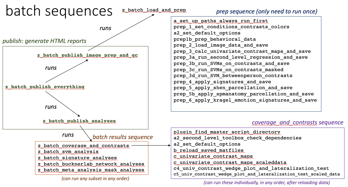
Step 5: Run batch scripts that publish date-stamped HTML reports
These run and save reports in the ‘published_output’ subfolder in your analysis directory This allows for archiving and records of the analysis history.
This batch script allows you to run a menu of different sets of results (contrasts, svm analyses, signature analyses, etc.) in any order: z_batch_publish_analyses.m
This batch script runs both the data load batch and all results: z_batch_publish_everything.m
These batch scripts are run in ‘publish’ scripts. You can run them on their own, too, but ‘set up paths’ and ‘reload’ first.
`z_batch_load_and_prep.m
z_batch_coverage_and_contrasts.m
z_batch_svm_analysis.m
z_batch_signature_analyses.m
z_batch_bucknerlab_network_analyses.m
z_batch_meta_analysis_mask_analyses.m`
(See the canlab_batch_flowchart image above.)
MORE INFO ABOUT HOW FILES AND VARIABLES ARE STORED
in ‘prep_’ scripts: image names, conditions, contrasts, colors, global gray/white/CSF values are saved automatically in a DAT structure
- Extracted fmri_data objects are saved in DATA_OBJ variables
Contrasts are estimated and saved in DATA_OBJ_CON variables
Files with these variables are saved automatically when you run the prep scripts.
meta-data are saved in image_names_and_setup.mat image data are saved in data_objects.mat
They are loaded automatically when you run
b_reload_saved_matfiles.m